ClusteredMutations: Looking for a (Mutation) Shower.
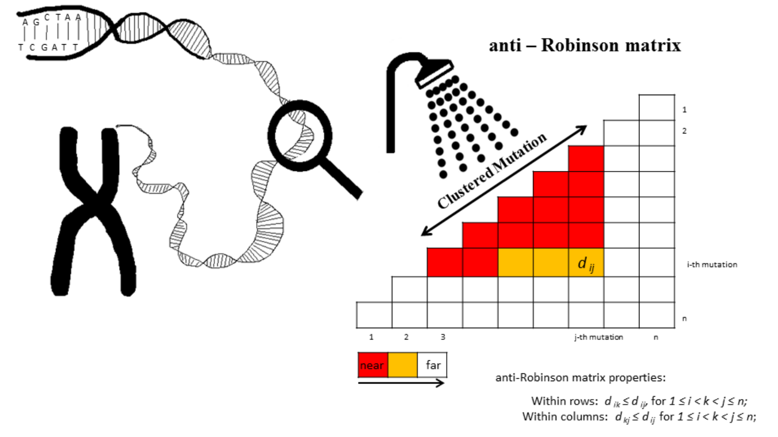
This vignette shows the steps to identify the hyper-mutated zones, i.e., groups of closely spaced mutations, with a data set of somatic substitution mutations from a primary breast cancer whole genome with a germline mutation in BRCA1 using ClusteredMutations.
keywords:
cancer genome, somatic mutation, mutation showers, clustered mutations, kataegis, anti-Robinson matrix
1 Example and applications.
In the following example, a data set (PD4107a) of somatic substitution mutations from a primary breast cancer whole genome with a germline mutation in BRCA1 [1, 4] is used to locate the hyper-mutated zones using ClusteredMutations.
First, ClusteredMutations package and PD4107a data set are loaded.
> library(ClusteredMutations)> data(PD4107a)showers() is called with a change in the default setting to identify the complex mutations. Complex mutations are those regions with two or more mutations with each mutation separated by less than 10 bp from their nearest neighbor; therefore, min=2 and max=10 are used. Because complex mutations likely originate from trans-lesion synthesis (TLS) past a single DNA lesion[3], Roberts et al.[6, 5] proposed treating them as a single event. In this example, all somatic substitution mutations are used, including complex mutations.
> data.showers<-showers(data=PD4107a, chr=Chr, position=Position, min=2, max=10)> head(data.showers, n=10)
chr pend pstart nend nstart distance number1 1 18331461 18331460 29 28 1 22 1 49584638 49584628 116 115 10 23 1 84702722 84702721 244 243 1 24 1 96832689 96832688 272 271 1 25 1 112246806 112246804 345 344 2 26 1 164753620 164753619 436 435 1 27 2 39902729 39902728 118 117 1 28 2 51867763 51867761 155 154 2 29 2 69402832 69402831 206 205 1 210 2 89459416 89459415 260 259 1 2The classic graph (Figure 1) to localize the regional clustering of mutations is the rainfall plot[4]. imd() permits the generation of a data set with the inter-mutational distance (IMD), the distance between each somatic substitution and the substitution immediately prior[4], and extra information, for example: base substitutions.
> extra <- factor(c(),levels=c("T>C","T>G","T>A","C>T","C>G","C>A"))
> extra[PD4107a$Ref_base=="A" & PD4107a$Mutant_base=="G"]<-"T>C"
> extra[PD4107a$Ref_base=="T" & PD4107a$Mutant_base=="C"]<-"T>C"
> extra[PD4107a$Ref_base=="A" & PD4107a$Mutant_base=="C"]<-"T>G"
> extra[PD4107a$Ref_base=="T" & PD4107a$Mutant_base=="G"]<-"T>G"
> extra[PD4107a$Ref_base=="A" & PD4107a$Mutant_base=="T"]<-"T>A"
> extra[PD4107a$Ref_base=="T" & PD4107a$Mutant_base=="A"]<-"T>A"
> extra[PD4107a$Ref_base=="G" & PD4107a$Mutant_base=="A"]<-"C>T"
> extra[PD4107a$Ref_base=="C" & PD4107a$Mutant_base=="T"]<-"C>T"
> extra[PD4107a$Ref_base=="G" & PD4107a$Mutant_base=="C"]<-"C>G"
> extra[PD4107a$Ref_base=="C" & PD4107a$Mutant_base=="G"]<-"C>G"
> extra[PD4107a$Ref_base=="G" & PD4107a$Mutant_base=="T"]<-"C>A"
> extra[PD4107a$Ref_base=="C" & PD4107a$Mutant_base=="A"]<-"C>A"
> PD4107a$extra<-extra
> rainfall<-imd(data=PD4107a,chr=Chr,position=Position,extra=extra)
> plot(rainfall$number, rainfall$log10distance, col=c("yellow", "green",
+ "pink", "red", "black", "blue")[rainfall$extra], pch=20,
+ ylab="Intermutation distance (bp)", xlab="PD4107a", yaxt="n")
> axis(2, at=c(0, 1, 2, 3, 4, 6), labels=c("1", "10", "100", "1000",
+ "10000", "1000000"), las=2, cex.axis=0.6)
> legend("topleft", legend = levels(rainfall$extra), col=c("yellow",
+ "green", "pink", "red", "black", "blue"), pch=20, horiz=TRUE,
+ text.font=4, bg='lightblue')
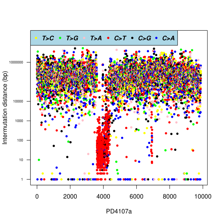
Figure 1 is the rainfall plot of PD4107a. The horizontal axis presents the number of consecutive mutations, the vertical axis indicates the distance between each somatic substitution and the substitution immediately prior (inter-mutational distance). Four features were observed in the rainfall plot of PD4107a (Figure 2):
1) Many of the somatic mutations have IMD greater than 10000 bp; thus, two consecutive mutations are sufficiently remote to be candidates to belong to the regional clustering of substitution mutations.
2) There were mutations with distances less than 10 bp, i.e., complex mutations[6, 5].
3) There were mutation zones with IMD less than 1000 bp on chromosomes 6 and 12. These zones can be hyper-mutated regions.
4) The preponderance of C>T and C>G substitutions is present in the candidate zones.
The rainfall plot identifies candidate hyper-mutated zones. Visual assessment can be erroneous (Figure 2). showers() is called with the default setting. There are no clustered mutations.
> set.seed(42)
> position<-c( c((runif(1001,min=1,max=10000001))),
+ c(c(10110001,10110011,10110021,10110031,10110041,10120000,
+ 10120001,10120011,10120021,10120031,10130000,
+ 10130001,10130011,10130021,10130031,10140000,
+ 10140001,10140011,10140021,10140031,10150000,
+ 10150001,10150011,10150021,10150031,10160000,
+ 10160001,10160011,10160021,10160031,10170000,
+ 10170001,10170011,10170021,10170031,10180000,
+ 10180001,10180011,10180021,10180031,10190000,
+ 10210001,10210011,10210021,10210031,10220000,
+ 10220001,10220011,10220021,10220031,10230000,
+ 10230001,10230011,10230021,10230031,10240000,
+ 10240001,10240011,10240021,10240031,10250000,
+ 10250001,10250011,10250021,10250031,10260000,
+ 10260001,10260011,10260021,10260031,10270000,
+ 10270001,10270011,10270021,10270031,10280000,
+ 10280001,10280011,10280021,10280031,10290000) +
+ round(runif(81,min=0,max=500))),
+ c(round(runif(991,min=10296000,max=20200000))))
> rainfall<-imd(position=position)
> #Rainfall plot for PD4107a cancer sample;
> plot(rainfall$number, rainfall$log10distance, pch=20,
+ ylab="Intermutation distance (bp)", xlab="Example", yaxt="n")
> axis(2, at=c(0, 1, 2, 3, 4, 6), labels=c("1", "10", "100", "1000",
+ "10000", "1000000"), las=2, cex.axis=0.6)
> theta <- seq(0, 2 * pi, length = 200)
> lines(x = 100 * cos(theta) + 1050, y = sin(theta) + 1.5, col="red")
showers() function in the example data set finds 0 hyper-mutated zones.
> showers(position=position)
[1] chr pend pstart nend nstart distance number<0 rows> (or 0-length row.names)showers() function in the PD4107a data set finds 21 hyper-mutated zones with 674 mutations, features() shows the mutation positions in the chromosome with additional information.
> showers(data=PD4107a,chr=Chr,position=Position)
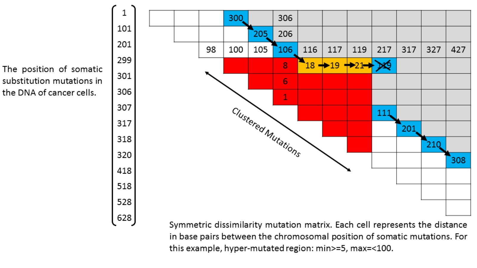
chr pend pstart nend nstart distance number1 6 126239586 126233148 466 370 6438 972 6 126279808 126274096 512 467 5712 463 6 126376071 126371860 525 513 4211 134 6 126394625 126392175 545 526 2450 205 6 126437625 126430855 708 546 6770 1636 6 130423519 130419337 797 740 4182 587 6 130438324 130433693 849 798 4631 528 6 130489124 130483574 887 851 5550 379 6 131796572 131788326 915 904 8246 1210 6 131818990 131810251 939 916 8739 2411 6 132401366 132396811 960 948 4555 1312 6 132552483 132544956 978 968 7527 1113 6 132603528 132599455 1025 979 4073 4714 6 133554257 133550552 1043 1038 3705 615 6 133716520 133707397 1066 1049 9123 1816 6 134025191 134015015 1088 1075 10176 1417 6 134118849 134115823 1096 1089 3026 818 6 135262041 135256447 1112 1104 5594 919 6 137982971 137979704 1133 1127 3267 720 6 138015423 138010978 1140 1134 4445 721 12 10508274 10505228 54 43 3046 12showers() function uses the anti-Robinson properties. For example, for a sample of DNA sequence of cancer cell with 14 somatic substitution mutations (Figure 3) and if the hyper-mutated zone contains those segments with >= 5 consecutive mutations with a distance of <= 100 bp, then:
1) the distance between the mutations 3 and 7 is
2) The distance is increased when moving away from the main diagonal, by row
and by column
3) The length of the hyper-mutated zone is determined by row or by column based on anti-Robinson properties: j - i + 1 = 10 - 4 + 1 = 7.
4) The calculated distance to the identified hyper-mutated zones is equal to: n - min + (number of the hyper-mutated zones in the sample) + 1 = 14 - 5 + 1 + 1 = 11.
> example1<-c(1,101,201,299,301,306,307,317,318,320,418,518,528,628)> 10**(dissmutmatrix(position=example1,upper=TRUE))
1 2 3 4 5 6 7 8 9 10 11 12 13 141 100 200 298 300 305 306 316 317 319 417 517 527 6272 100 100 198 200 205 206 216 217 219 317 417 427 5273 200 100 98 100 105 106 116 117 119 217 317 327 4274 298 198 98 2 7 8 18 19 21 119 219 229 3295 300 200 100 2 5 6 16 17 19 117 217 227 3276 305 205 105 7 5 1 11 12 14 112 212 222 3227 306 206 106 8 6 1 10 11 13 111 211 221 3218 316 216 116 18 16 11 10 1 3 101 201 211 3119 317 217 117 19 17 12 11 1 2 100 200 210 31010 319 219 119 21 19 14 13 3 2 98 198 208 30811 417 317 217 119 117 112 111 101 100 98 100 110 21012 517 417 317 219 217 212 211 201 200 198 100 10 11013 527 427 327 229 227 222 221 211 210 208 110 10 10014 627 527 427 329 327 322 321 311 310 308 210 110 100
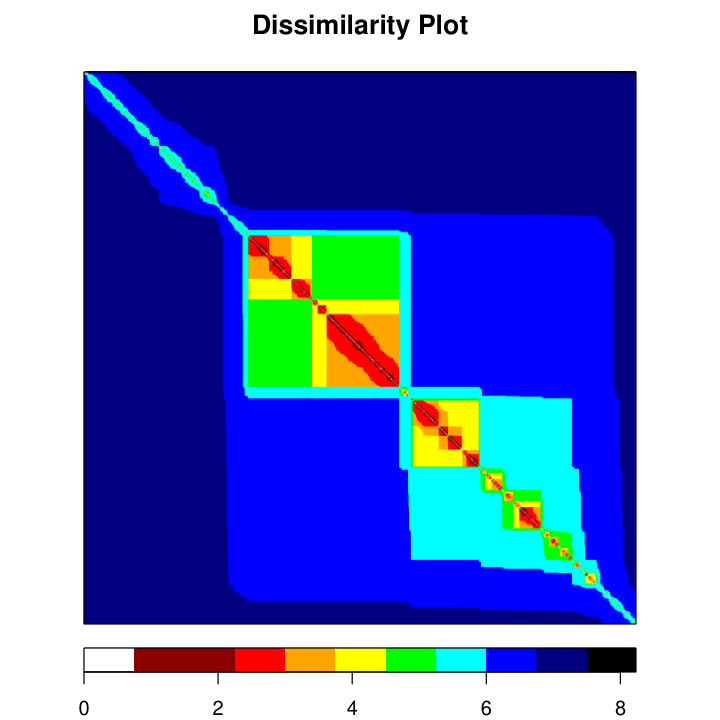
dissmutmatrix() obtains the symmetric dissimilarity mutations matrix. This function computes and returns the distance matrix computed using the Euclidean distance measure to compute the distances between all pairs of positions of somatic mutations. This matrix can be plotted using the dissplot() function of the seriation R package[2]. Plotting the distance matrix helps to visualize and identify mutation clusters in addition to locating the micro-clustered mutated regions within the macro-clustered mutated zones that occur during the oncogenic process. The plot is applied to chromosome 6 of the PD4107 data set (Figure 4). The distances, in logarithm of base 10, are colored according to the existing color palette. Observed clusters of mutations, or candidates for hyper-mutated zones (less than 5000 bp between distant mutations), are shown by orange and red squares (20 regions).
> mut.matrix <- dissmutmatrix(data=PD4107a, chr=Chr,
+ position=Position, subset=6)
> dissplot(mut.matrix, method=NA, options=list( col = c("black",
+ "navy", "blue", "cyan", "green", "yellow", "orange", "red",
+ "darkred", "darkred", "white")))
2 Conclusion.
The anti-Robinson matrix properties can be used to identify and view all small highly mutated zones within the oncogenic process. The properties of this matrix are implemented in an R package: ClusteredMutations.
References
- [1] (2013) Signatures of mutational processes in human cancer.. Nature 500 (7463), pp. 415–421. External Links: ISSN 1476-4687 0028-0836, Document Cited by: §1.
- [2] (2008) Getting things in order: an introduction to the r package seriation. 25 (1), pp. 1–34. External Links: ISSN 1548-7660, Link, Document Cited by: §1.
- [3] (2000) DNA polymerase zeta introduces multiple mutations when bypassing spontaneous DNA damage in saccharomyces cerevisiae.. 6 (6), pp. 1491–1499. External Links: ISSN 1097-2765 1097-2765 Cited by: §1.
- [4] (2012) Mutational processes molding the genomes of 21 breast cancers.. 149 (5), pp. 979–993. External Links: ISSN 1097-4172 0092-8674, Document Cited by: §1, §1.
- [5] (2013) An APOBEC cytidine deaminase mutagenesis pattern is widespread in human cancers.. 45 (9), pp. 970–976. External Links: ISSN 1546-1718 1061-4036, Document Cited by: §1, §1.
- [6] (2012) Clustered mutations in yeast and in human cancers can arise from damaged long single-strand DNA regions.. 46 (4), pp. 424–435. External Links: ISSN 1097-4164 1097-2765, Document Cited by: §1, §1.