Tutorial on modelling spatial and spatio-temporal non-Gaussian data with FRK
Abstract
In this vignette, we provide examples where we model non-Gaussian data using FRK version 2.x and above. All of the functionality that FRK offers in a Gaussian setting extends to a non-Gaussian setting: see the vignette “Introduction to FRK”, which describes how the BAUs and basis functions work; inference over different spatial manifolds (such as the sphere); inference in a spatio-temporal setting; and spatial change of support.
1 Methodology
The statistical model used by FRK in a non-Gaussian setting is a spatial generalised linear mixed (GLMM) model [Diggle et al., 1998], a hierarchical model consisting of two layers. In the process layer, we model the conditional mean of the data as a transformation of a latent spatial process, where the spatial process is modelled as a low-rank spatial random effects model; see Section 1.1. The process layer, which governs the conditional mean of the data, retains many similarities to that in previous versions of the package, as described by Zammit-Mangion and Cressie [2021] and in the vignette “FRK_intro”. In the data layer, we use a conditionally independent exponential-family model for the data; see Section 1.2. In Sections 1.3 and 1.4 we briefly discuss parameter estimation, and spatial prediction and uncertainty quantification.
1.1 The process layer
Denote the latent spatial process as , where indexes space in the spatial domain of interest . The model for is the so-called spatial random effects (SRE) model [Cressie and Johannesson, 2008],
| (1) |
where are spatially referenced covariates with associated regression parameters , is an -dimensional vector of pre-specified spatial basis functions with associated random coefficients , and is a fine-scale random process that is ‘almost’ uncorrelated.
FRK discretises the domain of interest into small, non-overlapping basic areal units (BAUs) such that . BAUs are a key element of FRK, as they provide a framework that allows one to use both point-referenced and areal data simultaneously, and one that facilitates the spatial change-of-support problem. After discretisation via the BAUs, we obtain the vectorised version of (1),
| (2) |
where is an -dimensional vector, and are known design matrices, and is the vector associated with the fine-scale process.
We model the fine-scale random effects as being independent and identically distributed Gaussian random variables with variance ; we model as a mean-zero multivariate-Gaussian random variable, typically using a sparse precision matrix parametrisation formualtion in a non-Gaussian setting.
Following standard generalised linear model theory [McCullagh and Nelder, 1989], FRK v.2 uses a link function, , to model as a transformation of the mean process, :
The mean process evaluated over the BAUs is
where is the inverse link function. An identity link function and a Gaussian data model yields the standard Gaussian FRK model.
1.2 The data layer
Given observations with footprints spanning one or more BAUs, we define the observation supports as for , where is a non-empty set in the power set of , and define . Let , . The vector of observations (the data vector) is then .
Since each is either a BAU or a union of BAUs, one can construct an matrix
where is the indicator function, which creates a linear mapping from to evaluations of the mean process over the observation supports;
| (3) |
The normalise_wts argument in SRE() controls whether the linear mapping of corresponds to a weighted sum or a weighted average; if normalise_wts = TRUE, then the weights are normalised so that the rows of sum to one, and the mapping represents a weighted average.
We assume that , where is a (nuisance) dispersion parameter and, for a generic random quantities and , denotes the probability distribution of given . That is, a given observation depends only on the value of the mean process at the corresponding observation support, rather than on the process over the whole domain. As a result, conditional on the latent spatial process, all observations are conditionally independent:
We model the conditional distribution as a member of the exponential family [McCullagh and Nelder, 1989, Sec. 2.2.2], with conditional expectation .
The model employed by FRK v.2 can be summarised as follows.
| (4) | |||
| (5) | |||
| (6) | |||
| (7) | |||
| (8) | |||
| (9) |
where is a known diagonal matrix with positive entries on the diagonal and is either unknown and estimated, or provided by the user.
1.3 Estimation
The complete-data likelihood function for our model is
| (10) |
where and are variance components, and its logarithm is
| (11) |
Under our modelling assumptions, the conditional density functions and are invariant to the specified link function and assumed distribution of the response variable. Of course, this invariance does not hold for . As we only consider data models in the exponential family, may be expressed as
| (12) |
where , , and are deterministic functions specific to the exponential family member, and is the canonical parameter.
The marginal likelihood, which does not depend on the random effects, is given by
| (13) |
where , and is the total number of random effects in the model. When the data are non-Gaussian, the integral in (13) is typically intractable and must be approximated either numerically or analytically. In FRK, we use the Laplace approximation, implemented using the R package TMB [Kristensen et al., 2016].
Given as input a C++ template function which defines the complete-data log-likelihood function (11), TMB [Kristensen et al., 2016] computes the Laplace approximation of the marginal log-likelihood, and automatically computes its derivatives, which are then called from within FRK by an optimising function specified by the user (nlminb() is used by default). TMB uses CppAD [Bell, 2005] for automatic differentiation, and the linear algebra libraries Eigen [Guennebaud et al., 2010] and Matrix [Bates et al., 2019] for vector and matrix operations in C++ and R, respectively; use of these packages yields good computational efficiency. TMB’s implementation of automatic differentiation is a key reason why we can cater for a variety of response distributions and link functions, as we do not need to consider each combination on a case-by-case basis.
1.4 Prediction and uncertainty quantification
There are three primary quantities of interest in this framework: The latent process , the mean process , and the noisy data process. To produce predictions and associated uncertainties, we need to determine the posterior distribution of these quantities.
It can be shown that the Laplace approximation implies that the posterior distribution of the random effects, is approximated to be Gaussian. This, in turn, implies that the posterior distribution of is also approximated to be Gaussian, and hence inference on can be done using closed form solutions. However, the posterior distribution of non-linear functions of (e.g., the mean process) are typically not available in closed form, and in this case some form of approximation is required. Hence, we choose to use a Monte Carlo (MC) framework.
For each quantity, we use the posterior expectation as our predictor. A commonly used metric for uncertainty quantification is the root-mean-squared prediction error (RMSPE). In a non-Gaussian setting, it can be difficult to interpret the RMSPE, and it is often more intuitive to quantify uncertainty through the width of the posterior predictive intervals. Hence, in FRK, we also provide the user with user-specified percentiles of the posterior predictive distribution. These quantities can be computed straightforwardly using MC sampling.
1.4.1 Arbitrary prediction regions
Often, one does not wish to predict over a single BAU, but over regions spanning multiple BAUs. Define the set of prediction regions as , where , and where is some non-empty set in the power set of . Like the data, the prediction regions may overlap. In practice, may not include entire BAUs; in this case, we assume that a prediction region contains a BAU if and only if there is at least some overlap between the BAU and the prediction region. Prediction over requires some form of aggregation across relevant BAUs. Since in the non-Gaussian setting aggregation must be done on the original scale, we restrict prediction over arbitrary regions to the mean (or the noisy data process). Therefore, predictions of the latent process are not allowed over arbitrary prediction regions.
Consider the predictions , where . These predictions are weighted sums of the predictions over the associated BAUs. Specifically,
where, in a similar fashion to the incidence matrix , the weights are optionally provided by the user in the wts field of the BAU object, and may be normalised if normalise_wts = TRUE. If wts is NULL, the BAUs are assumed to be equally weighted. Define . Since each element in is the union of subsets of , one can construct a matrix,
such that . Again, we use MC sampling to predict .
2 Example: Simulated Non-Gaussian, point-referenced spatial data
First, load the required packages.
library("FRK")       # for carrying out FRK
library("sp")        # for defining points/polygons
library("dplyr")     # for easy data manipulation
library("ggplot2")   # for plotting
Now, simulate some Poisson distributed spatial data.
m <- 250                                                   # Sample size
RNGversion("3.6.0"); set.seed(1)                           # Fix seed
zdf <- data.frame(x = runif(m), y= runif(m))               # Generate random locs
zdf$Y <- 3 + sin(7 * zdf$x) + cos(9 * zdf$y)               # Latent process
zdf$z <- rpois(m, lambda = exp(zdf$Y))                     # Simulate data
coordinates(zdf) = ~x+y                                    # Turn into sp object
There is an ‘expert’ way of using FRK that involves using the functions auto_BAUs() and auto_basis() to automatically construct BAUs and basis functions from the data, and SRE() and SRE.fit() to initialise and fit the SRE model object.
This ‘expert’ way is documented in the vignette “FRK_intro”.
Alternatively, there is a ‘simple’ way of using FRK that uses the high-level wrapper function FRK() that calls these functions under-the-hood; in this vignette, we will use the ‘simple’ way.
S <- FRK(f = z ~ 1,               # Formula to FRK
         list(zdf),               # All datasets are supplied in list
         nres = 2,                # Low-rank model to reduce run-time
         response = "poisson",    # data model
         link = "log",            # link function
         nonconvex_hull = FALSE)  # convex hull
pred <- predict(S)                # prediction stage
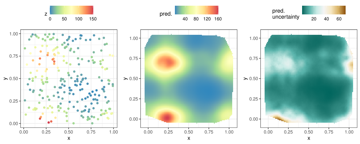
FRK includes two plotting methods, plot() and plot_spatial_or_ST(); the former takes an SRE object and the result of a call to predict, and returns a list of ‘ggplot’ objects containing the predictions and uncertainty quantification of those predictions, while the latter is a general-purpose function for ‘Spatial*DataFrame’ and ‘STFDF’ objects.
plot_list <- plot(S, pred$newdata)
plot_list <- c(plot_list, plot_spatial_or_ST(zdf, "z"))
This list of plot objects can then be arranged using one of the many functions for arranging ‘ggplot’ objects: See Figure 1.
## Ignoring unknown labels:
## * fill : "data"
3 Example: Lognormally distributed soil data, point and block-level predictions
Between 1954 and 1963, nuclear devices were detonated at Area 13 of the Nevada Test Site in the United States, contaminating the surrounding soil with the radioactive element americium (Am). In 1971, the Nevada Applied Ecology Group measured Am concentrations in a region surrounding Ground Zero (GZ), the location where the devices were detonated [Paul and Cressie, 2011]. The total number of measurements (including some that are collocated) is 212. In the following, we load this data set (supplied by FRK), and define GZ.
data("Am_data")
coordinates(Am_data) = ~ Easting + Northing # convert to sp object
GZ_df <- data.frame("Easting" = 219868.09, "Northing" = 285320.8)
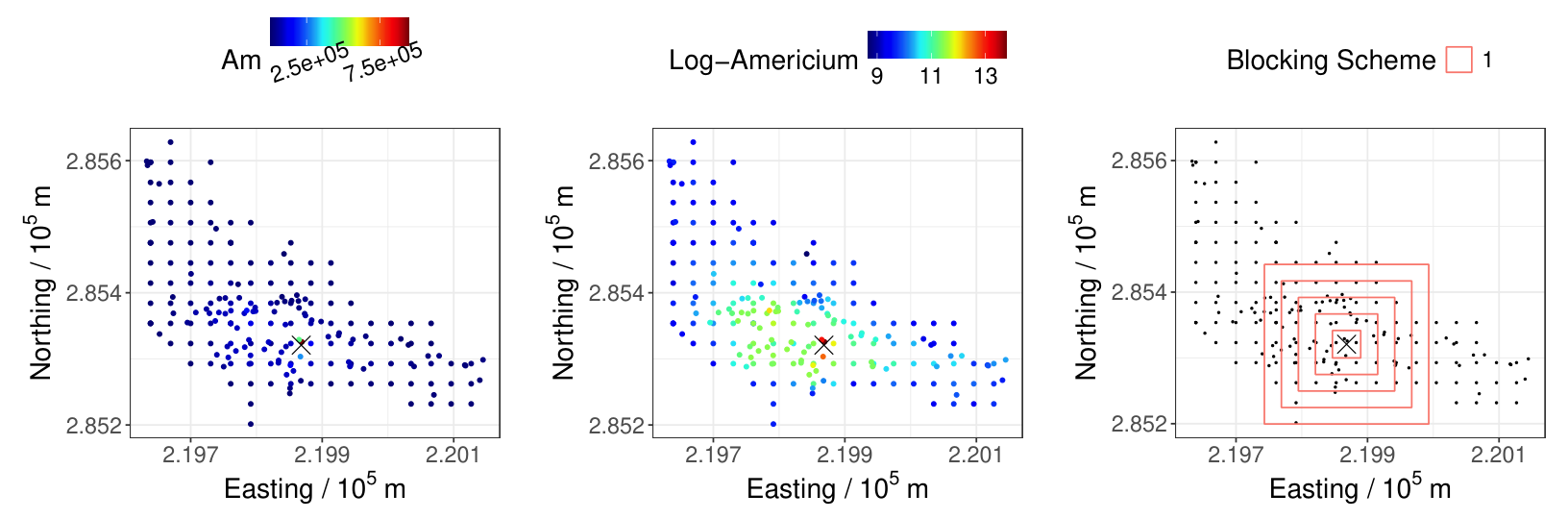
The left and centre panels of Figure 2 shows the data on the original scale and on the log scale, respectively. Paul and Cressie [2011] note that these Am concentrations are lognormally distributed, and that soil remediation is often made by averaging the contaminant over pre-specified spatial regions of called blocks. Hence, this application requires lognormal prediction over blocks, a task well suited to FRK. The right panel of Figure 2 shows a blocking scheme containing five blocks that we will predict over, which is centred on GZ.
Following Paul and Cressie [2011], we use a piecewise linear trend, where observations within a distance of 30.48m from GZ follow a different trend to those observations beyond 30.48m from GZ. In FRK, covariates must be defined at the BAU level.
BAUs <- auto_BAUs(manifold = plane(),
                  type = "grid",
                  data = Am_data,
                  nonconvex_hull = FALSE)

## Add covariates to the BAUs
d_cutoff <- 30.48
d_BAU <- distR(coordinates(BAUs), GZ_df)
BAUs$x1 <- as.numeric(d_BAU < d_cutoff)
BAUs$x2 <- d_BAU * BAUs$x1
BAUs$x3 <- as.numeric(d_BAU >= d_cutoff)
BAUs$x4 <- d_BAU * (BAUs$x3)
In the following, we indicate that a scalar covariance matrix should be used for the fine-scale variation term (implicit when allowing FRK() to construct that BAUs), and we replicate lognormal kriging by fixing the measurement-error standard deviation to a small value. Then, we run FRK() as usual, set est_error = FALSE so that the measurement-error standard deviation is not estimated.
BAUs$fs     <- 1
Am_data$std <- 1

S <- FRK(f = Am ~ -1 + x1 + x2 + x3 + x4, data = list(Am_data),
         response = "gaussian",
         link = "log",
         BAUs = BAUs,
         nres = 2,
         est_error = FALSE)
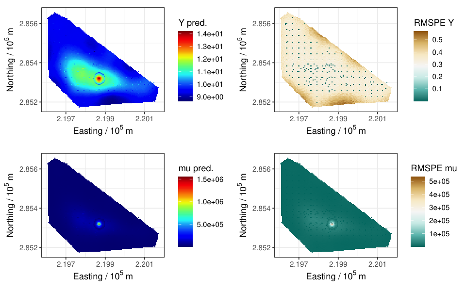
By predicting over the BAUs, one may generate predictions over the entire spatial domain. In predict(), we set type = c("link", "mean") to obtain predictions for both the latent process , and the mean process . Figure 3 shows BAU level predictions and uncertainty using FRK.
pred <- predict(S, type = c("link", "mean"))
plot_list <- plot(S, pred$newdata)
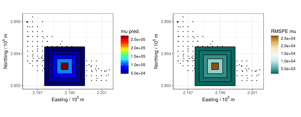
Alternatively, by passing a ‘SpatialPolygonsDataFrame’ object into the newdata argument of predict(), one may straightforwardly generate block-level predictions. When predicting over arbitrary spatial regions, FRK is limited to prediction of the mean process.
pred <- predict(S, newdata = blocks)
These block level predictions may be plotted with the help of SpatialPolygonsDataFrame_to_df(); see Figure 4.
References
- Matrix: sparse and dense matrix classes and methods. Note: R package version 1.2-17 External Links: Link Cited by: §1.3.
- CppAD: a package for C++ algorithmic differentiation.. Note: https://coin-or.github.io/CppAD/doc/cppad.htmAccessed: 2019-06-15 Cited by: §1.3.
- Fixed rank kriging for very large spatial data sets. Journal of the Royal Statistical Society 70, pp. 209–226. Cited by: §1.1.
- Model-based geostatistics. Journal of the Royal Statistical Society 47, pp. 299–350. Cited by: §1.
- Eigen v3. Note: https://libeigen.gitlab.io/Accessed: 11-05-2019 Cited by: §1.3.
- TMB: Automatic differentiation and Laplace approximation. Journal of Statistical Software 70, pp. 1–21. Cited by: §1.3, §1.3.
- Generalized Linear Models. Chapman & Hall, London, UK. Cited by: §1.1, §1.2.
- Lognormal block kriging for contaminated soil. European Journal of Soil Science 62, pp. 337–345. Cited by: §3, §3, §3.
- FRK: an R package for spatial and spatio-temporal prediction with large datasets. Journal of Statistical Software In press. Cited by: §1.