An Introduction to PottsUtils
Package PottsUtils comprises several functions related to the Potts models defined on undirected graphs. The main purpose of the package is to make available several functions that generate samples from the models. To facilitate that, there are other utilities. Furthermore, there is a by-product of simulation functions. Altogether, there are three sets of functions. The first produces basic properties of a graph to facilitate the simulation functions (they maybe used for other purposes as well). The second provides various simulation functions. The third currently includes only one function which computes the normalizing constant based on simulation results.
This introduction was intended to help users to understand better the functions, the documentation (Rd files), and the source code. For more technical details (mathematical proof among others), we refer users to references herein.
Hereafter, first we introduce some basic concepts and definitions related to the Potts models. Second, algorithms used in simulation functions are presented in a concise way. Third, a function to obtain normalizing constant is introduced. Forth, we discuss some computational issues. Finally, some future work is outlined.
1 Notation and Terminology
In this section we introduce concepts and definitions involved in the discussions of the Potts models. The notations used are similar to those given in Winkler (2003). Based on that, several related functions in the package are introduced.
We consider the Potts model defined on a finite undirected graph. A graph describes a set of connections between objects. Each object is called a node or vertex. There are observations to characterize the properties of vertices. Let be a finite set, the set of vertices; , where is the total number of vertices. For every vertex , let take values in a finite set of categories , where is the number of categories. In the package we use different colors to represent different categories and vertices from the same category are of the same color. The product is the space of configurations . A strictly positive probability measure on for every is called a stochastic or random field. Note that has to be strictly positive on to satisfy the assumptions of the Hammersley-Clifford theorem; see Besag (1974) and Winkler (2003) for details.
A collection of subsets of is called a neighborhood system, if (i) and (ii) if and only if . The sites are called neighbors of . We use to denote that and are neighbors of each other. There is an edge between and if and only if they are neighbors. Define a graph , where is the set of edges. For a finite undirected graph, the number of vertices are finite and edge is equivalent to edge . The function getEdges() can be used to get edges of a graph. When neighbors and are from the same category (of the same color), then there is a bond between them.
The random field is a Markov random field (MRF) w.r.t. the neighborhood system if for all ,
Probability measures of the form
are called Gibbs fields (or measures). is called the energy function or Hamiltonian, and is called the partition function or normalizing constant. For detailed account on MRF, Gibbs measures, and related issues, we refer to Winkler (2003).
When using Markov random field models, the first question is how to define neighbors of all vertices. For a 1D lattice, the simplest way to define neighbors is that every vertex (except those on the boundaries) has the two adjacent vertices as its neighbors, see Figure 1 for illustration. Of course, a vertex could have more than two neighbors.

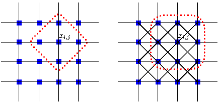
For a 2D lattice, there are two common ways to define neighbors. One is that neighbors of a vertex comprise its available N, S, E, and W adjacencies. Another is that, besides those four, there are four diagonal adjacencies on its north-west, north-east, south-west, and south-east. See Figure 2 for illustrations. Probability measures defined on the former are called the first-order Markov random fields and the latter the second-order Markov random fields.
For a 3D lattice, besides defining six neighbors in the , , and directions, one can add twelve diagonal neighbors in the , , and planes, and another eight on the 3D diagonals. This leads to a six neighbor structure, an eighteen neighbor structure, and a twenty-six neighbor structure. For illustration, see Figure 3.
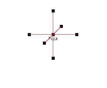
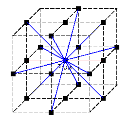
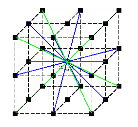
The package provides a function called getNeighbors() to generate all neighbors of a graph.
After defining neighbors, the second question is how to model the spatial relationship among neighbors. One choice is to use a model from the Potts model family, a set of MRF models with the Gibbs measure defined as follows.
| (1) |
where is a normalizing constant and indicates neighboring vertices. We need to define neighborhood structure and then assign relationships among neighboring vertices. The parameter , called the inverse temperature, determines the level of spatial homogeneity between neighboring vertices in the graph. A zero would imply that neighboring vertices are independent. We use positive values. The are weights and we assume . The term is called the external field. The are functions of . When , the external field completely characterizes the distribution of the independent .
When model (1) becomes
| (2) |
For , this model is called the Ising model (Ising, 1925); for it is the Potts (1953) model. The Ising model was originally proposed to describe the physical properties of magnets. Due to its flexibility and simplicity, the Ising model and its various versions have been widely used in other fields, such as brain models in cognitive science (Feng, 2008), information and machine learning theory (MacKay (2003) and references therein), economics (Bourgine and Nadal (2004) and references therein), sociology (Kohring, 1996) and game theory (Hauert and Szabó, 2005).
The most commonly used Potts model is the one without an external field and with ,
| (3) |
We refer to this as the simple Potts model.
Let and . Then (1) reduces to
| (4) |
where is the weight between vertex and . For example we might take where is a distance function, say Euclidean distance, between two vertices. This model is referred to as the compound Potts model.
In model (1), let and define as
| (5) |
where . We call this model the repulsion Potts model. This model assumes an ordering of the colors and that neighboring vertices are most likely of the same color, and if they are different then it is more likely that they are similar than totally different. See Feng (2008) for more details.
2 Simulation of the Potts Models
It is very hard to find algorithms (such as inversion of CDF, rejection sampling, adaptive rejection sampling, or ratio-of-uniforms sampling) to generate i.i.d. samples from the Potts models, and Markov chain methods have to be used for the simulation.
To generate samples from model (1), single site updating, for example Gibbs sampling, is easy but may mix slowly. The Swendsen and Wang (1987) algorithm (SW) is widely used to generate random samples from the simple Potts model. Wolff’s algorithm (Wolff, 1989) has been advocated as an alternative to the SW. A Gibbs sampler that takes advantage of the conditional independence structure to update variables , could make the simulation much faster than a single site updating scheme (Feng, 2008). When there is external field, the partial decoupling method might outperform the Gibbs sampling.
2.1 Swendsen-Wang Algorithm
The SW algorithm was originally proposed for the simulation of the simple Potts model. Drawing auxiliary variables for neighboring vertices from independent and uniform distributions on makes the joint density
| (6) |
The conditional distribution of given is also uniform on possible configurations. If , then there is a bond between vertices i and j (when definitely ); otherwise there is no further constraint. Therefore, all vertices can be divided into patches (clusters). A patch is a collection of vertices, in which any two vertices are connected by a bond or a sequence of bonds. There is no bond between vertices from different patches. See Figure 4 for illustrations. The vertices within each patch should belong to the same category and the categories of different patches are i.i.d. from the discrete uniform distribution among all possible categories.
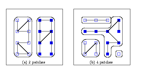
The SW algorithm is the seminal work on algorithms using auxiliary variables (in this case ) in this area. A slightly generalized version of the original SW algorithm can be used to generate samples from a compound Potts model (Feng, 2008). Given all vertices, there are three steps in each iteration as follows.
- 1.
Build bonds among vertices in neighbor with probability
- 2.
Build patches for vertices bonded together
- 3.
Flip the patches randomly to any color
The SW algorithm may outperform single-site updating samplers, especially when there is no external field and there is patchiness among vertices, in which simultaneous switching of clusters is necessary. For more details see Feng (2008).
2.2 Wolff’s Algorithm
A modification of the Swendsen-Wang algorithm was proposed by Wolff (1989). The difference between the Wolff and the SW is that instead of flipping all patches randomly, one patch is chosen and all vertices in that patch are flipped to their opposites in the simple Potts model. To be more specific, for Wolff’s algorithm, a vertex, say , is selected randomly among all vertices, and bonds between and its neighbors are set the same way as in the SW. If there are bonds between and its neighbors, say , then the bonds between vertices in and their neighbors are set. Follow the same procedure recursively until no new bonds are created. Now there is a patch around and all vertices in this patch are flipped to their opposites. Note, there is no randomness involved when flipping vertices for the Ising Model. Although Wolff’s algorithm is similar to the SW, its proof is formalized from another perspective where detailed balance and irreducibility are verified (see Wolff (1989) for details).
To generate samples from a compound Potts model, a slighted generalized version of the original Wolff algorithm as follows can be adopted. There are four steps in each iteration.
- 1.
Randomly select a vertex
- 2.
Build a patch around it with probability
- 3.
Continue building the patch till no additional vertex can be bonded together
- 4.
Flip the patch randomly to another color
See Feng (2008) for more details.
2.3 A Gibbs Sampler Using Conditional Independence
Various multiple-site sampling methods might outperform single-site updating, but sometimes they might not. Multi-site sampling methods like the SW algorithm could tackle the critical slowing down problem. When there is no external field, from the results pointed out in Higdon (1998), the SW algorithm outperforms single-site Metropolis updating when is at the critical value. When there is an external field (a likelihood function in Bayesian inference for example), the SW slows down since it does not make good use of the data. Hurn (1997) and Smith and Smith (2006) suggested that when is large, Gibbs samplers might be more effective. The choice of the best sampling method is likely to be problem-specific and there is no clear-cut winner as pointed out in Hurn (1997) and Higdon (1998). Furthermore, the previous studies just focus on relatively small grids in two dimensions with the number of categories equal to 2. What the convergence properties of various algorithms are on a three dimensional large grid with more than 2 categories, the case in MRI analysis for example (Feng, 2008), needs further study. Given that, a Gibbs sampler might be a good choice under certain circumstances. The package provides functions that uses the Gibbs sampler taking advantage of the conditional independence structure to update colors of vertices. It could make the simulation much faster than a one-site-after-another sampling scheme by using the vectorization functions in .
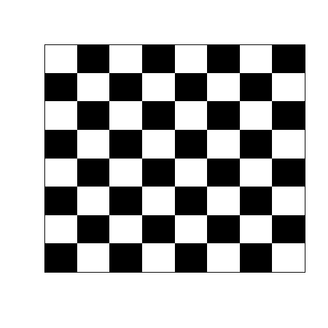
The idea is that if we can divide variables that need to be updated into different blocks and given the variables in other blocks, all the variables within the same block are conditionally independent, then we can update all blocks iteratively with the variables within the same block being updated simultaneously. In Figure (a) of 5, under the four neighbor structure in 2D, given the black vertices, the whites are independent and vice versa. By this kind of independence, updating can be done in two steps: one for the blacks, one for the whites. The idea of taking advantage of this kind of independence can be traced back at least to the “Coding Methods” in Besag (1974). It was described in Wilkinson (2005) and detailed discussion can be found in Winkler (2003). This conditional independence can be generalized to 3D lattices with a six neighbor structure, see (b) of Figure 5 for illustration. Under six neighbor structure, given the blacks, the whites are independent and vice versa. The minimum number of blocks to make the vertices within each block independent given the other blocks is called the chromatic number in Winkler (2003). So the chromatic numbers for four neighbor configuration in 2D and six neighbor in 3D are both 2.
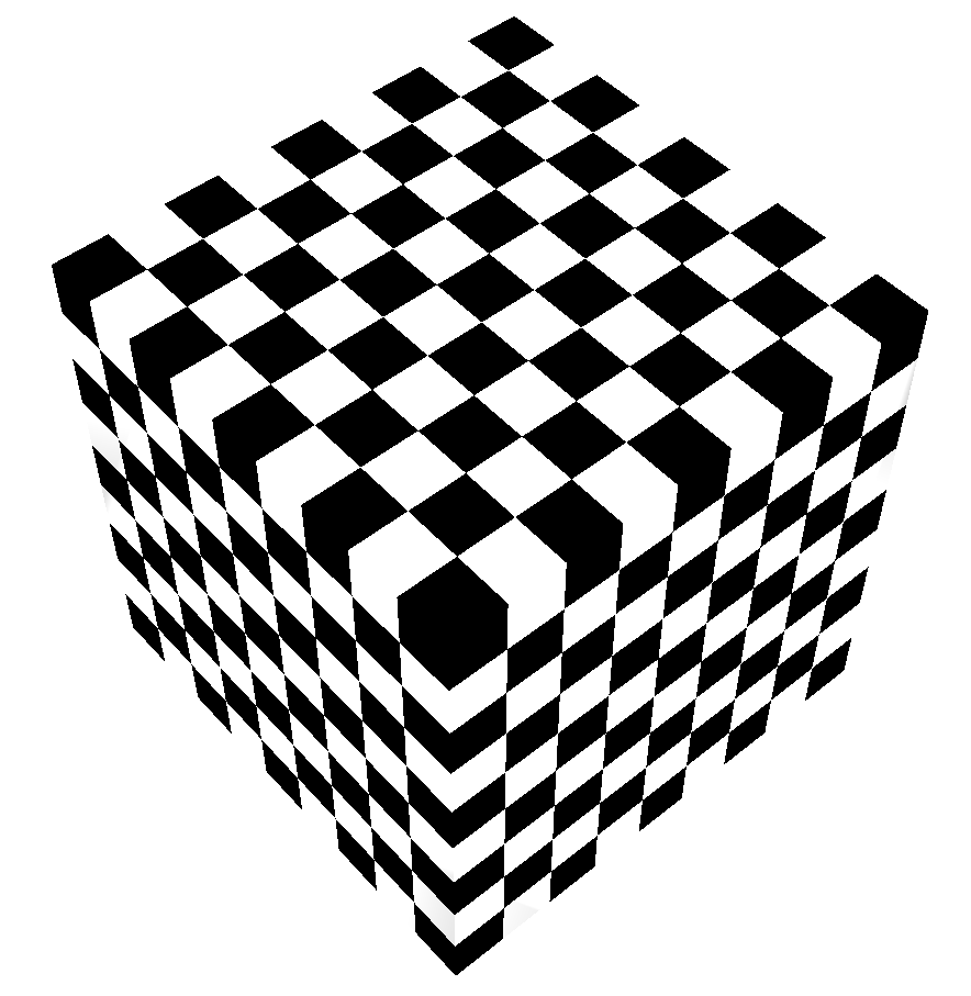
The extension to the eight neighbor configuration in 2D and eighteen and twenty-six neighbor in 3D is as follows. Under the eight neighbor structure in 2D, the chromatic number is four; under the eighteen neighbor configuration in 3D, the chromatic number is seven; under the twenty-six neighbor configuration in 3D, the chromatic number is eight. For more details, see Feng (2008).
The function to split vertices into conditional independent blocks is getBlocks(). Right now, for a 2D graph, the vertices can be divided into either 2 or 4 blocks, and for a 3D graph either 2 or 8. The functions using the Gibbs sampler that takes advantage of conditional independence are BlocksGibbs() and rPotts1(). The difference between the two is that the first one can only generate samples from a Potts model without the external field while the second is good for all Potts models. The relationship among neighboring vertices can be defined by specifying the parameter spatialMat.
2.4 The Partial Decoupling Method
Besides the Gibbs sampling, another way to obtain samples from a Potts model with external field is to use the partial decoupling method through the function rPotts1().
The partial decoupling method was originally developed by Higdon (1993) for an Ising model with an external field. Given the external field, the symmetry property is violated. Instead of drawing for neighbor points from independent uniform distributions on , draw from the uniform distribution . Now, the bonding probability is not only controlled by alone, but as well. When , it reduces to single site updating; when , it corresponds to the SW algorithm. The smaller the , the less likely bonds are formed. After setting the bonds, clusters are usually not independent anymore and Gibbs, Metropolis-Hastings, or even partial decoupling could be used to update the coarser model. The Gibbs sampling is used in the package.
The goal of choosing is to improve the mixing when sampling from . Strategies for the determination of are based on the nature of the likelihood function of the data. For example, choosing for vertices on the boundaries of adjacent sub-graphs and for others can prevent the clusters from growing beyond certain limits. Another choice is with , where and are observations for vertex and . The details of the partial decoupling method can be found in Higdon (1998) and Hurn (1997).
3 Calculation of the Normalizing Constant
The normalizing constant is not critical and can be ignored if is known. However, if is treated as unknown, for example in studies using the Bayesian methods (Green and Richardson, 2002; Smith and Smith, 2006), then the normalizing constant is necessary when drawing samples from the conditional distribution of by a Metropolis-Hastings algorithm.
The package provide a function getNC() to obtain the normalizing constant of a simple Potts model. The method adopted is similar to that in Green and Richardson (2002) and Smith and Smith (2006), in which the thermodynamic integration approach was used. The thermodynamic integration approach comes from the differential equations for describing thermodynamic relationships in physics. Basically, the thermodynamic integration method uses the fact that the normalizing constant can be obtained by solving the differential equation
where and is the number of categories. Since
it follows
| (7) |
In order to compute we use the following steps:
- 1.
Take grid values . For each , obtain simulations of the graph and estimate by the average of the functions from simulations. Possible methods for simulation include Gibbs sampling with single site updating, or the SW, or the Wolff algorithms discussed previously.
- 2.
Compute the integral by numerical integration.
4 Computational Issues
As mentioned in sub-section 2.3, it is beneficial to use vectorization functions in to fulfill the idea of conditional independence. Furthermore, for the SW algorithm the major computational work is the identification and labeling of the patches of connected vertices. This is an instance of a connected component labeling problem for an undirected graph. We use Rem’s algorithm (Dijkstra, 1976) to fulfill the task in the function getPatches(). Besides facilitating the SW algorithm, it can be used in other clustering methods as well. See Heller et al. (2006) for example.
5 Future Work
In the future, the package might be upgraded in several directions. First we might incorporate more available sampling methods for the Potts models. Second, the speed of current functions might be enhanced by using embedded functions and parallel computations. Third, changes based on feedback of users.
References
- Spatial interaction and the statistical analysis of lattice systems (with discussion). Journal of the Royal Statistical Society. Series B (Methodological) 36 (2), pp. 192–236. Cited by: §1, §2.3.
- P. Bourgine and J. P. Nadal (Eds.) Cognitive economics-and interdisciplinary approach. Springer. Cited by: §1.
- A discipline of programming. Englewood Cliffs, New Jersey : Prentice-Hall, Inc. Cited by: §4.
- Bayesian hidden markov normal mixture models with application to MRI tissue classification. Ph.D. Thesis, The University of Iowa. Cited by: §1, §1, §2.1, §2.2, §2.3, §2.3, §2.
- Hidden markov models and disease mapping. Journal of the American Statistical Association 97, pp. 1055–1070. Cited by: §3, §3.
- Game theory and physics. American Journal of Physics 73 (5), pp. 405–414. Cited by: §1.
- Cluster-based analysis of fmri data. NeuroImage 33, pp. 599–608. Cited by: §4.
- Comments on “Spatial Statistics and Bayesian Computation”. Journal of the Royal Statistical Society Series B-Statistical Methodology 55 (1), pp. 78. Cited by: §2.4.
- Auxiliary variable methods for Markov chain Monte Carlo with applications. Journal of the American Statistical Association 93, pp. 585–595. Cited by: §2.3, §2.4.
- Difficulties in the use of auxiliary variables in Markov chain Monte Carlo methods. Statics and Computing 7, pp. 35–44. Cited by: §2.3, §2.4.
- Beitrag zur theorie des ferromagnetismus. Zeitschrift fu̇r Physik 31, pp. 253–258. Cited by: §1.
- Ising models of social impact: the role of cumulative advantage. Journal de Physique I 6 (2), pp. 301–308. Cited by: §1.
- Information theory, inference and learning algorithms. Cambridge University Press. Cited by: §1.
- Some generalized order-disorder transformations. In Cambridge Philosophic Society, Vol. 48, pp. 106–109. Cited by: §1.
- Estimation of binary Markov random fields using Markov chain Monte Carlo. Journal of Computational and Graphical Statistics 15 (1), pp. 207–227. Cited by: §2.3, §3, §3.
- Nonuniversal critical dynamics in monte carlo simulations. Physical Review Letters 58 (2), pp. 86–88. Cited by: §2.
- Parallel bayesian computation. In Handbook of Parallel Computing and Statistics, E. J. Kontoghiorghes (Ed.), pp. 481–512. Cited by: §2.3.
- Image analysis, random fields and dynamic monte carlo methods: a mathematical introduction. second edition, Springer-Verlag. Cited by: §1, §1, §1, §2.3.
- Collective monte carlo updating for spin systems. Physical Review Letters 62 (4), pp. 361–364. Cited by: §2.2, §2.