Haplotype enrichment in tropical maize
Matthias Frisch
1 Prepare and phase the populations
Load the tropical maize data
We consider 264 tropical maize lines from CIMMYT’s Drought Tolerance Maize for Africa project that were analyzed with 1135 SNP markers. Data from Crossa et al. (2010). The original marker data are available from the Genetics webpage. Thanks to Dr. Jose Crossa and Dr. Raman Babu for providing the map data and the permission to use this data set as an example for data analysis.
The tropical maize data are distributed with the package. We keep the original data and create a separate working copy for filtering.
> data("v-tropmaize-vcf")> st.load.vcf.data(+ v.tropmaize.vcf,+ data.set = "base"+ )> st.copy.marker.data("clustering", "base")
Filter markers and lines
Retain biallelic markers with at most 10% missing genotypes.
> st.restrict.marker.data(+ NoAll.MAX = 2, # At most two alleles per marker+ MaMis.MAX = 0.1, # Missing-call limit per marker+ data.set = "clustering"+ )Remove lines with more than 10% missing genotypes, then retain markers with expected heterozygosity of at least 0.1.
> st.restrict.marker.data(+ InMis.MAX = 0.1, # Missing-call limit per line+ data.set = "clustering"+ )> st.restrict.marker.data(+ ExHet.MIN = 0.1, # Retain polymorphic, informative markers+ data.set = "clustering"+ )Obtain statistics for the filtered markers and list the available datasets.
> filtered <- st.marker.data.statistics(+ data.set = "clustering",+ gen = FALSE # Omit the large genotype table+ )> st.data.set.list()
Define five clusters
Calculate the Rogers distance matrix from the filtered marker data.
> dist.mat <- st.genetic.distances(+ measure = "rd", # Rogers distance between lines+ format = "m", # R 'dist' object for cmdscale+ data.set = "clustering"+ )Apply k-means to its rows using a fixed seed to reproduce the five clusters.
> set.seed(1) # Reproduce the random starts and cluster labels> clus <- kmeans(+ as.matrix(dist.mat), # Rows are distance profiles, not SNPs+ centers = 5,+ nstart = 25 # Keep the best of 25 random starts+ )> clusters <- clus$clusterCalculate principal coordinates for the figure and display the cluster sizes.
> pco <- cmdscale( # Principal coordinates from Rogers distances+ dist.mat,+ k = 4, # Retain four axes; plot the first two below+ eig = TRUE # Keep eigenvalues to assess the embedding+ )> PC <- pco$points> print(table(clusters))
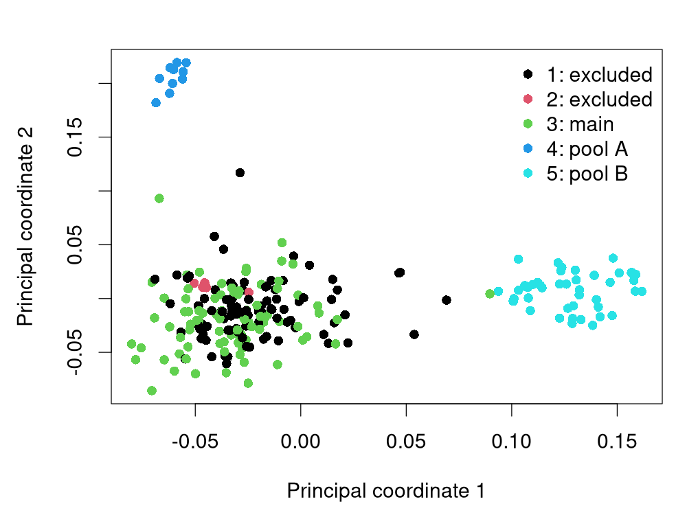
clusters 1 2 3 4 590 6 83 10 43The first two principal coordinates show the five clusters with the same plotting settings used for the selected-donor comparison below.
> plot(+ PC[, 1],+ PC[, 2],+ col = cluster.colours[clusters], # Stable cluster colours+ pch = 16,+ xlab = "Principal coordinate 1",+ ylab = "Principal coordinate 2"+ )
Choose the main and donor populations
The green cluster 3 is the base population. Cluster 4 (blue) supplies pool A and cluster 5 (light green/turquoise) supplies pool B. Clusters 1 and 2 are excluded. Both pools are derived from the same marker data, so marker identities, maps and allele coding agree.
> main.ind <- names(clusters)[clusters == 3]> a.pool <- names(clusters)[clusters == 4]> b.pool <- names(clusters)[clusters == 5]> pools <- list(A = sort(a.pool), B = sort(b.pool))> joint.ind <- c(main.ind, a.pool, b.pool)Summarize the cluster identities and line counts of the three populations.
> populations <- data.frame(+ Population = c("Main", "A", "B"),+ Cluster = c(3, 4, 5),+ Lines = c(length(main.ind), length(a.pool), length(b.pool))+ )> print(populations, row.names = FALSE)
Population Cluster Lines Main 3 83 A 4 10 B 5 43
Create separate marker datasets
Copy the filtered dataset and retain only the base-population lines.
> st.copy.marker.data("base.phased", "clustering")> st.restrict.marker.data(ind.list=main.ind, data.set="base.phased")Copy the filtered dataset and retain only the lines in donor pool A.
> st.copy.marker.data("A.phased", "clustering")> st.restrict.marker.data(ind.list=a.pool, data.set="A.phased")Copy the filtered dataset and retain only the lines in donor pool B.
> st.copy.marker.data("B.phased", "clustering")> st.restrict.marker.data(ind.list=b.pool, data.set="B.phased")
Phase the base population
The tropical maize accessions are inbred lines, and we use st.phase here only to impute missing marker calls. Their predominantly homozygous genotypes leave little ambiguity about phase. Each population is processed separately with a fixed seed, and impute=TRUE retains the inferred calls at missing marker genotypes.
> st.phase(+ impute = TRUE, # Retain inferred calls at missing genotypes+ phasing.options = list(seed = 20261003), # Reproducible calls+ data.set = "base.phased"+ )
Phase donor pool A
Use a separate, reproducible seed for the first donor pool.
> st.phase(+ impute = TRUE, # Retain inferred calls at missing genotypes+ phasing.options = list(seed = 20261004),+ data.set = "A.phased"+ )
Phase donor pool B
Apply the same phasing settings to the second donor pool.
> st.phase(+ impute = TRUE, # Retain inferred calls at missing genotypes+ phasing.options = list(seed = 20261005),+ data.set = "B.phased"+ )
2 Enrichment using haplotyping options
Define haplotyping options once
This workflow uses non-overlapping windows of five adjacent markers. Short terminal windows are retained, and no block crosses a chromosome boundary. The same options are reused in every call; blocks are defined from the base population, so selecting donors cannot change their borders.
> haplotype.options <- list(+ hap = 5,+ hap.unit = 1 # Block size is measured in markers+ )
Select five donors from pool A
Forward selection adds the donor with the greatest remaining gain at each of five steps. Shared variants count once per block. With exclude.compatible=TRUE, variants compatible with incomplete base calls are excluded from the score. The returned genotype names follow selection order.
> # Shared donor variants count once in the combined gain.> forward.A <- st.select.enrichment(+ base.pool = "base.phased",+ enrichment.pool = "A.phased",+ n = 5,+ haplotype.options = haplotype.options,+ exclude.compatible = TRUE,+ method = "forward"+ )> print(forward.A)
[1] "228" "213" "232" "217" "218"
Create the selected donor dataset
Copy and restrict the donor pool using those names.
> st.copy.marker.data("selected.A", "A.phased")> st.restrict.marker.data(ind.list=forward.A, data.set="selected.A")
Calculate enrichment from the selected lines
Calculate the additional block-specific haplotypes contributed jointly by the five selected lines.
> gain.A <- st.calculate.enrichment(+ base.pool = "base.phased",+ enrichment.pool = "selected.A", # Only the five chosen donors+ haplotype.options = haplotype.options,+ exclude.compatible = TRUE # Exclude uncertain additions+ )> print(gain.A$summary, row.names = FALSE)
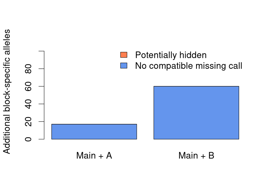
Base.lines Enrichment.lines Main Additional Hidden No.match Score 83 5 2218 17 0 17 17 Enriched Gaining.blocks 2235 16
The printed summary contains the following quantities.
- •
Base.lines: Number of lines in the base population used for the comparison. Here all 83 phased base lines are retained, and both stored homologues of each line contribute to the haplotype catalogue. This is a count of individuals; the diversity they represent is reported separately in Main.
- •
Enrichment.lines: Number of donor lines included in the enrichment calculation. Here the donor dataset contains the five selected lines from pool A, rather than all ten candidates. Both homologues contribute, but a variant carried by several selected donors is counted only once within its block.
- •
Main: Number of distinct complete haplotypes observed in the base population, summed over all blocks; here the total is 2218. Repeated copies within one block count once, while variants at different blocks count separately. Incomplete haplotypes do not enter this observed-allele count.
- •
Additional: Number of distinct complete donor haplotypes absent from the complete base calls at the corresponding blocks. The five donors supply 17 such variants, each counted once per block. This total includes both uncertain and unambiguous additions, so it equals Hidden + No.match.
- •
Hidden: Number of additional variants compatible with at least one incomplete base homologue at all its observed markers. Such variants may already occur where base calls are missing and are excluded from the present score. Here the count is zero because the imputed base haplotypes contain no missing calls.
- •
No.match: Number of additional variants incompatible with every incomplete base haplotype at the corresponding block. These variants are absent from complete base calls and cannot be hidden in incomplete calls. Here all base calls have been imputed, so all 17 additional variants fall into this category.
- •
Score: Number of additional variants credited by the selection criterion; here the score is 17. With exclude.compatible=TRUE, it equals No.match. The Hidden count is zero in this example, so including compatible variants would give the same score, equal to Additional.
- •
Enriched: Total number of distinct complete haplotypes represented after combining the base population and selected donors. It is calculated as Main + Additional, giving here. Shared variants count once within their block, regardless of how many base or donor lines carry them.
- •
Gaining.blocks: Number of blocks with at least one additional observed donor haplotype; here 16 blocks gain diversity. Each block counts once, even if it contains several additional variants. Blocks whose additions are all classified as hidden also count, because this quantity is based on Additional.
Select five donors from pool B
Repeat the same analysis for the second pool, retaining the same base population and options.
> # Keep the same base and blocks for a comparable pool-B gain.> forward.B <- st.select.enrichment(+ base.pool = "base.phased",+ enrichment.pool = "B.phased",+ n = 5,+ haplotype.options = haplotype.options,+ exclude.compatible = TRUE,+ method = "forward"+ )> print(forward.B)
[1] "140" "156" "175" "133" "154"
Copy pool B and retain only the five selected donor lines.
> st.copy.marker.data("selected.B", "B.phased")> st.restrict.marker.data(ind.list=forward.B, data.set="selected.B")
Calculate enrichment from pool B
One additional allele means one additional variant at one block, not at every block. The two pool comparisons remain separate; their gains must not be added because they may introduce the same variants.
> gain.B <- st.calculate.enrichment(+ base.pool = "base.phased",+ enrichment.pool = "selected.B", # Only the five chosen donors+ haplotype.options = haplotype.options,+ exclude.compatible = TRUE # Exclude uncertain additions+ )> print(gain.B$summary, row.names = FALSE)
Base.lines Enrichment.lines Main Additional Hidden No.match Score 83 5 2218 60 0 60 60 Enriched Gaining.blocks 2278 51
Inspect individual blocks
The detailed tables identify where enrichment occurs and which sequences are added. The examples below display their first rows; complete results remain in the returned objects.
> print(head(gain.B$by.block), row.names = FALSE)> print(head(gain.B$alleles), row.names = FALSE) # Added sequences
Block Main Hidden No.match Additional Score Enriched b000000 10 0 0 0 0 10 b000001 13 0 2 2 2 15 b000002 12 0 1 1 1 13 b000003 17 0 0 0 0 17 b000004 18 0 3 3 3 21 b000005 10 0 1 1 1 11 Block Sequence Hidden b000001 1;2;1;1;2 FALSE b000001 1;1;2;1;2 FALSE b000002 2;1;2;1;1 FALSE b000004 1;2;1;2;1 FALSE b000004 1;1;2;2;1 FALSE b000004 2;2;2;2;1 FALSE
3 Enrichment using fixed block borders
Define and retain the block borders
Construct explicitly the same non-overlapping five-marker blocks used above, retaining short terminal blocks at chromosome ends.
> blocks <- st.def.hblocks(+ hap = 5,+ hap.unit = 1, # Block size is measured in markers+ data.set = "base.phased"+ )Display the first five block definitions, including their marker membership.
> print(head(blocks, 5), row.names = FALSE)
Chrom Pos Name Class 1 3.5672 b000000 b 1 7.1442 b000001 b 1 11.1725 b000002 b 1 13.9740 b000003 b 1 22.8237 b000004 b Markers PZA036132;PZA036131;PZA036142;PZA036141;PZA003931; PZA003934;PZB019151;PZA035181;PZA035191;PZA035201; PZA035203;PZA035204;PZA035211;PZA035511;PZA035521; PZA035583;PZA035571;PZA036631;PZA036622;PHM165331; PZB007186;PZA0035812;PZD000971;PZA029219;PZB025153;
A table with the same Name, Chrom and Markers columns can also be constructed or imported to use arbitrary block borders. The Markers column lists marker names separated by semicolons. Each block must contain consecutive markers on one chromosome, block names must be unique, and blocks must not overlap.
Select donors using the fixed blocks
Supply this table to select five donors from pool A, using the same block borders and enrichment criterion as in the earlier example.
> forward.fixed.A <- st.select.enrichment(+ base.pool = "base.phased",+ enrichment.pool = "A.phased",+ n = 5,+ blocks = blocks,+ exclude.compatible = TRUE,+ method = "forward"+ )> print(forward.fixed.A)
[1] "228" "213" "232" "217" "218"
4 Comparison of the two pools
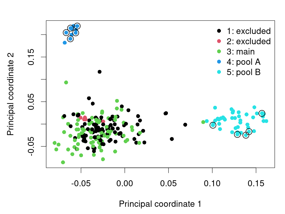
The principal-coordinate plot shows the five clusters, with circles marking the five selected donors from each pool.
The bar chart shows the additional block-specific haplotype alleles supplied by the five selected donors from each pool.
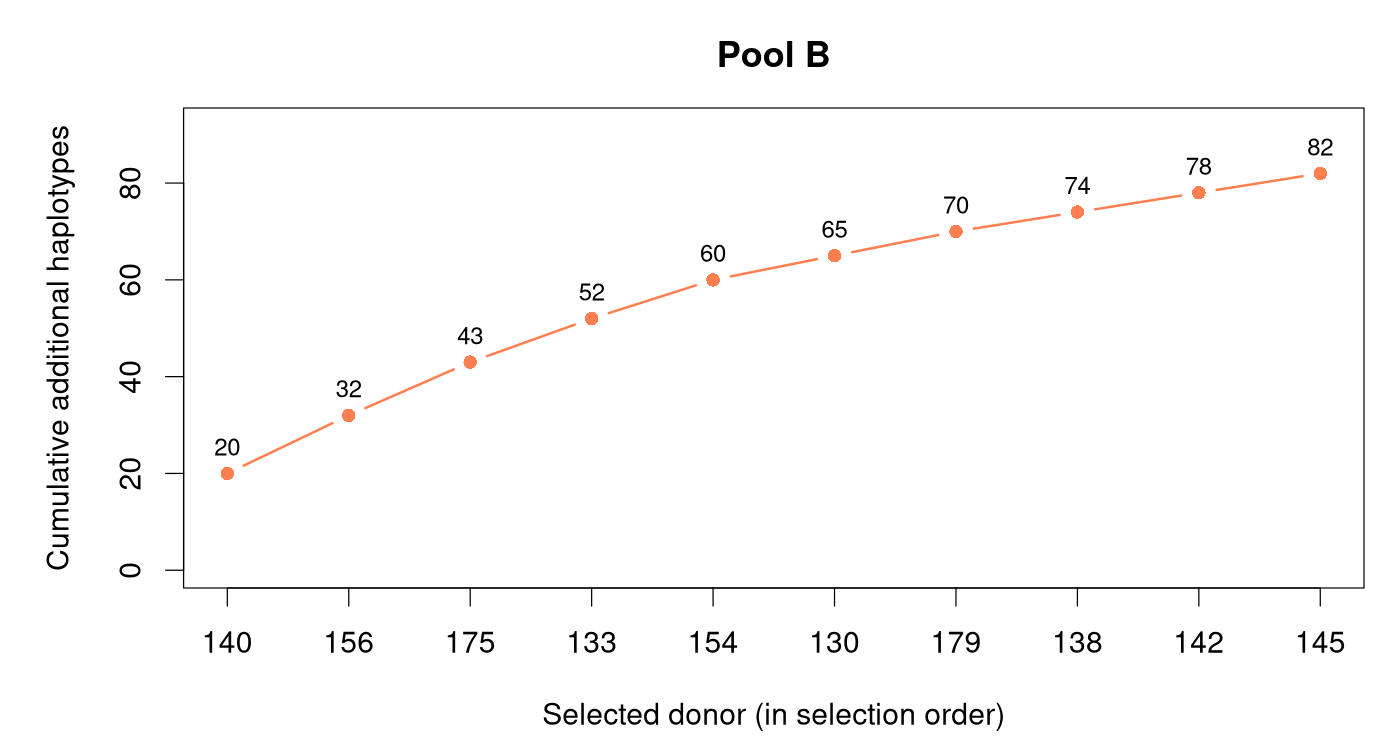
Cumulative enrichment along ten selected donors
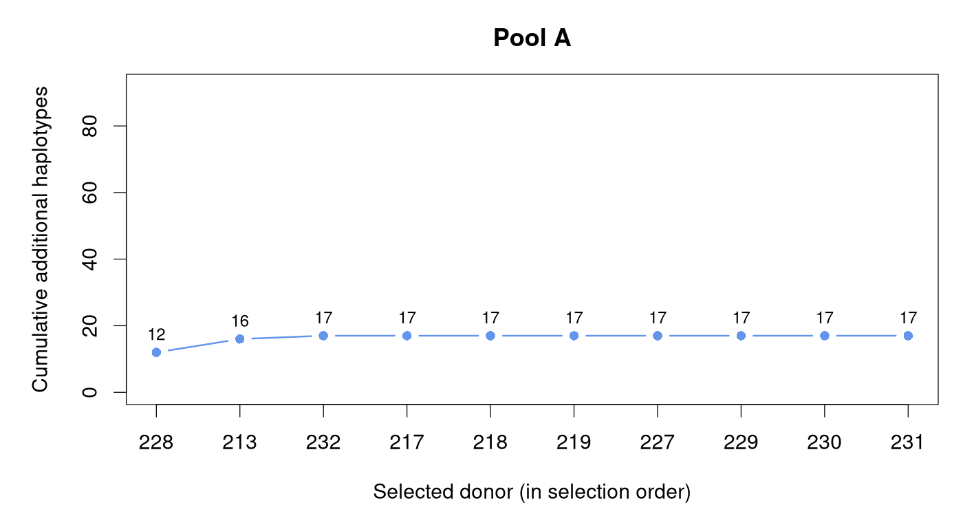
The curves extend forward selection to ten donor lines from each pool, using the same 83 base lines and five-marker block borders as above. The horizontal axis identifies donors in selection order; the vertical axis shows the cumulative additional block-specific haplotypes after each donor is included. Shared variants count once within each block, and both plots use the same vertical scale. The fifth point reproduces the corresponding five-donor enrichment total.
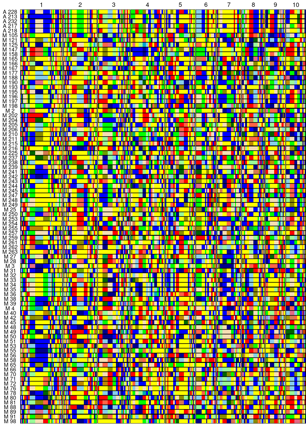
Five-marker blocks: base plus pool A
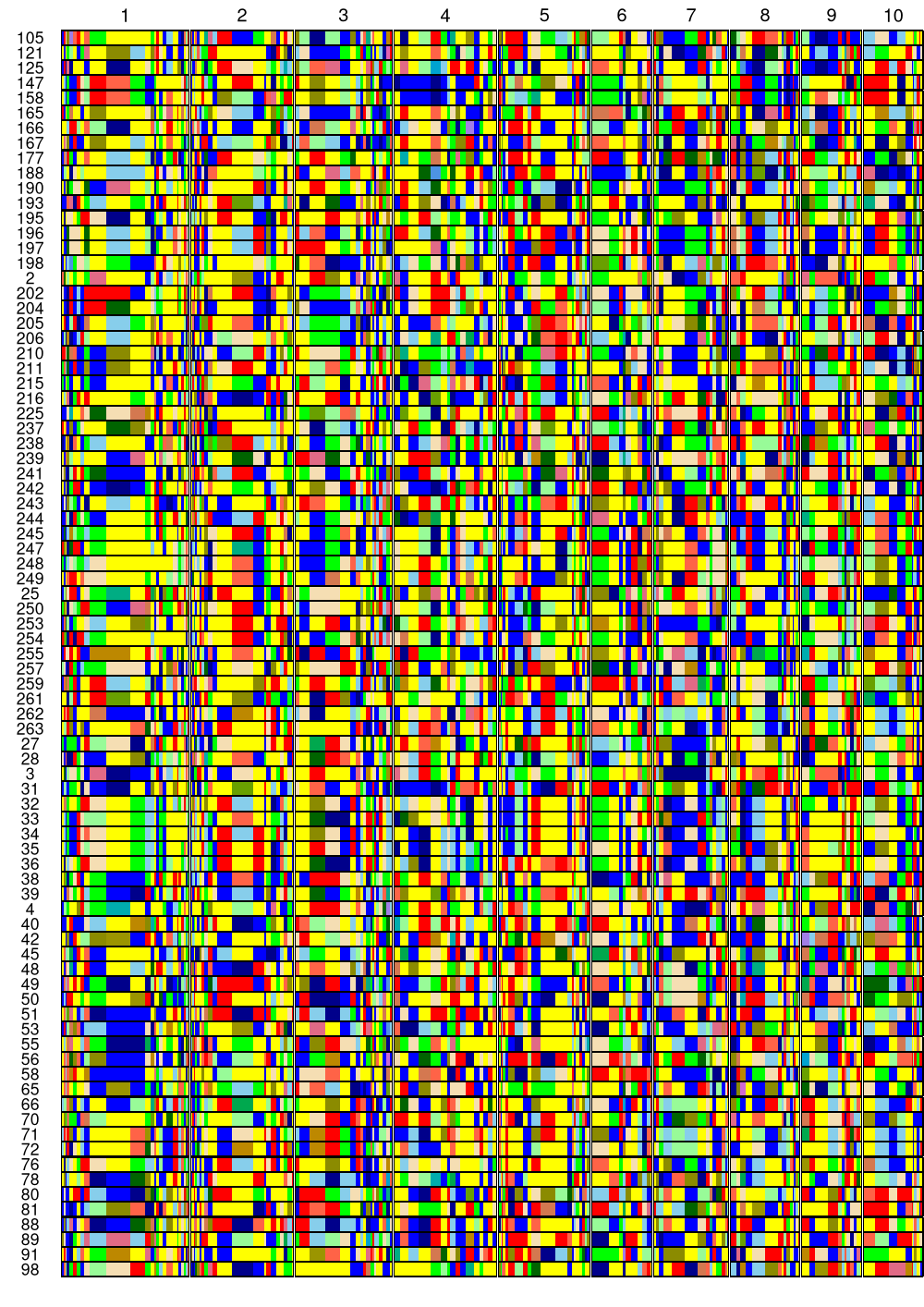
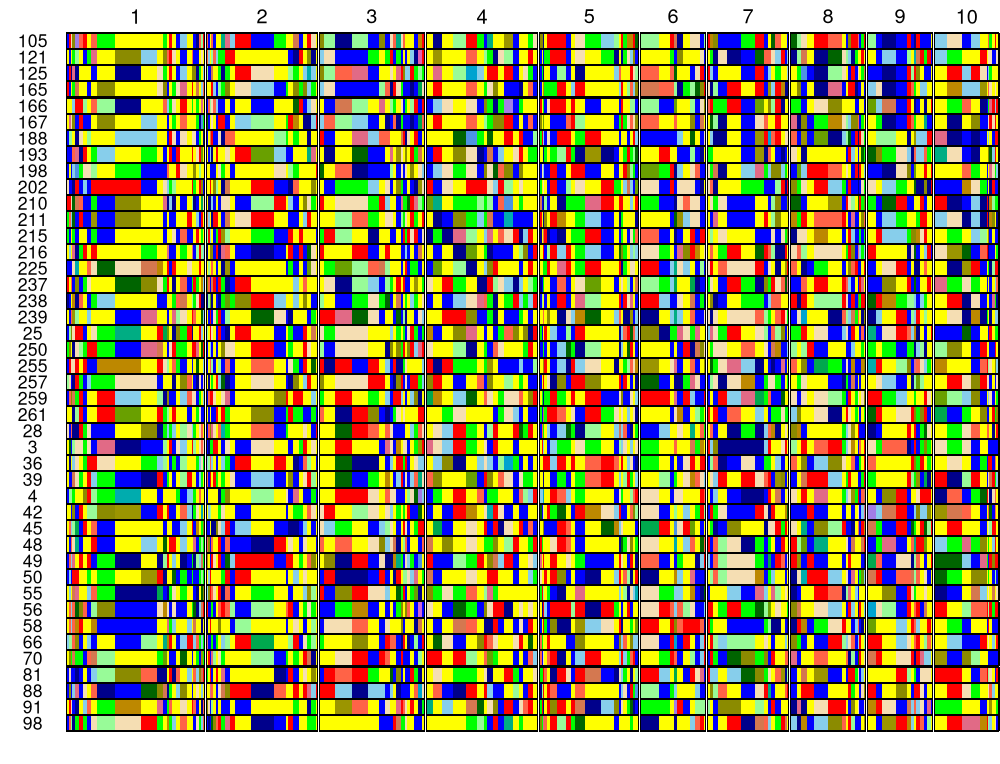
The five selected A lines appear at the top, followed by all 83 lines from base.phased, the same base population used for enrichment. Chromosomes 1–10 run from left to right. Colours identify variants within each block: yellow is the most frequent complete allele and blue the second most frequent across the base and both donor pools. The same colour mapping is used in both graphical-genotype figures.
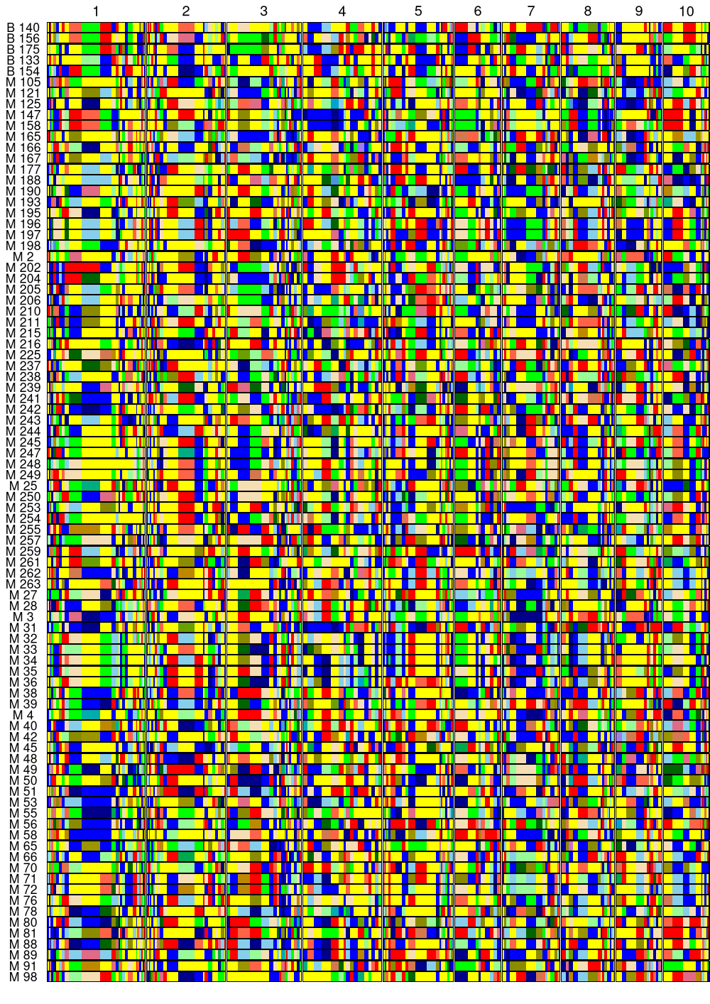
Five-marker blocks: base plus pool B
The five selected B lines appear at the top, followed by the 83 lines from the same base.phased dataset, in the same order as in the preceding figure. The allele-to-colour mapping is also unchanged.
5 Build a core collection by forward selection
st.detect.core builds a core collection from one phased population. Here the candidates are the same 83 base lines used for enrichment, and we reuse the same five-marker block borders. Forward selection starts with an empty core and adds the line contributing the largest number of previously unrepresented qualifying haplotypes at each step.
Allow all base lines as an upper limit; selection stops earlier if no remaining line provides a positive gain.
> core <- st.detect.core(+ pool = "base.phased",+ n.max = length(base.ids),+ blocks = blocks,+ exclude.compatible = TRUE,+ method = "forward"+ )The returned genotypes list contains the nested selected line sets. The segments vector reports their cumulative numbers of distinct complete haplotypes, counted separately for each block. Shared sequences count once within a block. The block borders remain fixed.
Tabulate the number of included lines and represented haplotypes, showing the first three steps and the final core size.
> core.curve <- data.frame(+ Lines = lengths(core$genotypes), # Each entry is the whole core+ Haplotypes = core$segments # Cumulative, not marginal gains+ )> print(rbind(head(core.curve, 3), tail(core.curve, 1)),+ row.names = FALSE)
Lines Haplotypes 1 169 2 321 3 452 80 2218
The plot shows the percentage of complete block-specific haplotypes represented by each core, relative to all haplotypes in the full base population. Horizontal guides mark 80% and 90% coverage; vertical guides identify the smallest cores reaching those levels: 30 and 43 lines, respectively. Steps reflect the inclusion of whole lines.
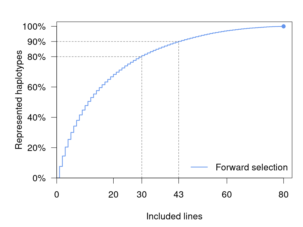
The final 80 lines represent all 2218 complete block-specific haplotypes observed in the 83-line base population.
Original population for core selection
All 83 lines in base.phased represent 2218 complete block-specific haplotypes. Chromosomes 1–10 run from left to right, using the same five-marker blocks and allele colours as in the pool-comparison figures.
Core population retaining 90% of haplotypes
The 43 forward-selected lines represent 1999 of the 2218 haplotypes (90.1%). The lines retain their order from the original-population plot; block borders, allele colours and the height of each genotype row are unchanged.
6 Literature review and methodological comparison
Selection of individuals that collectively represent genetic variation has long been a central problem in the conservation and utilization of genetic resources. Allelic richness provides a direct criterion when the objective is to retain distinct variants rather than reproduce their population frequencies. Schoen and Brown (1993) investigated sampling strategies that maximize the number of alleles represented in collections of fixed size. Their work established the value of marker information for allocating limited sampling resources. Gouesnard et al. (2001) subsequently implemented the maximization of allelic or phenotypic richness in MSTRAT. These studies provide the conceptual basis for selecting complementary individuals: accessions carrying variants already represented contribute less additional richness than accessions carrying previously unrepresented variants.
Retention of a predefined collection during subsequent expansion also has a precedent in plant genetic resources. Le Cunff et al. (2008) used MSTRAT to construct nested grapevine core collections from SSR genotypes. A core of 48 varieties represented the alleles retained after excluding the rarest variants. This collection was then retained as the starting set for an extension to 92 varieties that captured all 326 SSR alleles in the original collection. The additional accessions therefore supplied diversity absent from an existing core. Although this application concerned individual SSR loci and sought complete coverage, it demonstrates that augmentation of a fixed collection according to missing alleles is an established strategy.
Haplotype-based selection has been developed extensively for allocating sequencing resources. Druet et al. (2014) investigated the selection of individuals for whole-genome sequencing and its consequences for genotype imputation and genomic prediction. Their AHAP approaches used haplotypes inferred from SNP-panel information to increase the diversity represented by the sequenced individuals. The AHAP* criterion assigned equal weight to rare and common haplotypes. This provides a close precedent for an objective based on the number of distinct haplotypes rather than solely on pedigree relationships or the frequency of common variants. The target was a sequencing reference set, however, rather than the incremental contribution of donors to a specified breeding population.
Bickhart et al. (2016) addressed redundancy in sequencing panels using nonoverlapping marker segments in Holstein cattle. Their iterative AHAP2 procedure selected an individual, removed its covered haplotypes from further consideration, and recalculated the scores of the remaining candidates. Their inverse-weight selection procedure applied the same iterative principle while favouring lower-frequency haplotypes. The main selection analyses considered homozygous haplotypes above a frequency threshold and sought the smallest set of animals covering those targets. The repeated removal of covered variants is directly relevant to forward selection: the contribution of each subsequent candidate is conditional on the individuals already chosen.
Gonen et al. (2017) implemented a related strategy in AlphaSeqOpt. Haplotypes of a specified number of markers were defined from phased data, their frequencies were calculated, and focal individuals were selected successively. After each selection, the chosen individual’s haplotypes were masked in the remaining population. Repetition produced a specified number of focal individuals. The procedure favoured frequent haplotypes because sequencing them facilitates imputation in many other individuals. A further component allocated sequencing resources among focal individuals and their relatives. This application combines marker-window haplotypes, a sample-size constraint, and conditional selection, but its frequency and sequencing objectives differ from an unweighted count of additional variants.
Joint optimization of haplotype representation has also been formulated using integer programming. Cheng et al. (2021) represented haplotype carriage by a binary incidence matrix and identified a minimum set of animals containing all target haplotypes. Their complete-coverage problem was solved exactly, whereas a further formulation for limited sequencing resources included frequency-based scores and restrictions on redundancy. These formulations show how collective haplotype representation can be addressed by combinatorial optimization. The distinction between minimizing the number of individuals required for complete coverage and maximizing coverage for a fixed number of individuals remains important, as these are different optimization problems.
In crop improvement, haplotypes also provide a basis for identifying useful variation and choosing complementary donors. Brinton et al. (2020) developed a haplotype-led framework for wheat breeding that connected characterization of genomic diversity with its targeted exploitation. Sanchez et al. (2025) investigated the incorporation of genetic resources into elite flint maize and used a haplotype criterion based on estimated breeding values. Their forward donor-selection procedure accounted for complementarity with recipients and previously introduced donors. These studies connect haplotype information with breeding decisions, although the value of a haplotype for a trait and its contribution to variant richness are distinct quantities. A previously absent variant need not have a favourable agronomic effect.
The enrichment approach presented here applies these principles to a fixed base population and a separate pool of candidate donors. Both populations are phased before selection and evaluated using common block borders. The borders can be generated from haplotyping options applied to the base population or supplied explicitly, for example after an LD-based analysis of that population. For block , let denote the set of haplotypes represented in the base population and the set carried by donor . For a selected donor set , additional haplotype richness is
Both homologues contribute when a donor is heterozygous. Each distinct additional haplotype is counted once within its block, irrespective of the number of selected donors carrying it. An increase of one therefore means one additional block-specific variant, not one additional variant in every block. The count must also be distinguished from the number of blocks that gain at least one variant: a single block can contribute several additions.
This objective is a haplotype-level form of allelic-richness maximization. A haplotype block can be regarded as a multiallelic locus whose alleles are phased marker sequences. Keeping the base population fixed makes selection conditional on diversity already available, as in the extension of nested core collections. Relative to sequencing-panel applications, the relevant variants are those absent from the base, and each eligible addition has the same weight. Relative to trait-oriented donor selection, no estimated marker or haplotype effects enter the criterion. Separate donor pools can thus be compared for their potential contribution of additional diversity, provided that the marker coding and block definitions are comparable.
Incomplete haplotypes require an explicit distinction between observed absence and uncertain absence. Complete donor haplotypes can be compared with complete base haplotypes directly. When exclusion of compatible variants is requested, a donor haplotype that matches the observed markers of an incomplete base homologue is not credited as an unambiguous addition in the selection score. This conservative rule acknowledges that the variant may already be present but partially unobserved. Its eligibility assessment is fixed relative to the original base population. Phasing and imputation quality nevertheless affect the inferred sequences, and the resulting enrichment is conditional on those inferred data and on the chosen block resolution.
With fixed blocks and eligibility rules, each donor supplies a fixed set of eligible block-specific variants absent from the base. Selection then maximizes the size of the union of these sets. The objective is monotone and submodular: adding a donor cannot reduce coverage, and its marginal contribution cannot increase as more donors are selected. Best-subset search determines a globally optimal set when completed, whereas forward selection repeatedly adds the donor with the greatest remaining marginal contribution. The latter need not attain the optimum. Applying the result of Nemhauser et al. (1978), its coverage satisfies
For five donors the bound is approximately 0.672. This is a worst-case bound under the stated fixed-set assumptions, not an expected efficiency or evidence that a particular selected set is optimal.
6.1 Comparison with the approach presented here
The connection to core-collection methods is the maximization of represented allelic richness, with each fixed haplotype block treated as a multiallelic locus. In st.detect.core, the collection starts empty and each selected line adds previously unrepresented block-specific haplotypes. In st.select.enrichment, the existing base population is retained and candidate donors are scored for the variants they add to it. This second task follows the same conditional-extension principle illustrated by the nested grapevine collections of Le Cunff et al. (2008), where a previously selected core was retained during expansion. Here the counted alleles are complete phased marker sequences within common blocks.
Haplotype-based sequencing studies also seek complementary individuals and reduce repeated coverage of the same variants. Bickhart et al. (2016) examined sequencing-panel selection with haplotype-frequency weighting; the present enrichment criterion gives each eligible additional block-specific haplotype the same weight. Forward selection then updates the gain against the union already represented by the base and selected donors. The cumulative enrichment curves and the core-coverage curve make this shared coverage principle explicit, while the fixed base catalogue determines which variants qualify as additions.
The donor-selection procedure of Sanchez et al. (2025) likewise evaluates candidates in relation to recipients and donors already introduced. Their haplotypic estimated breeding values connect complementarity to predicted performance. The criterion used here measures complementarity through variant identity: a donor contributes when it supplies an eligible haplotype absent from the current collection. Its output can therefore serve as a diversity component in donor choice alongside trait-based criteria, with the consequences for agronomic performance evaluated separately.
The present workflow therefore combines established coverage and complementarity principles with an explicit comparison between phased base and donor populations, flexible common block definitions, and exact or forward search under the same enrichment criterion. Its output quantifies diversity available in the combined collection. It does not predict the transmission or retention of those variants through crossing, recombination and selection, nor does it establish an expected agronomic gain. Those consequences require additional genetic and breeding criteria.
References
Bickhart DM, Hutchison JL, Null DJ, VanRaden PM, Cole JB (2016) Reducing animal sequencing redundancy by preferentially selecting animals with low-frequency haplotypes. Journal of Dairy Science 99:5526–5534.
Brinton J, Ramirez-Gonzalez RH, Simmonds J, Wingen L, Orford S, et al. (2020) A haplotype-led approach to increase the precision of wheat breeding. Communications Biology 3:712.
Cheng H, Xu K, Li J, Abraham KJ (2021) Optimizing sequencing resources in genotyped livestock populations using linear programming. Frontiers in Genetics 12:740340.
Crossa J, de los Campos G, Pérez P, Gianola D, Burgueño J, et al. (2010) Prediction of genetic values of quantitative traits in plant breeding using pedigree and molecular markers. Genetics 186:713–724.
Druet T, Macleod IM, Hayes BJ (2014) Toward genomic prediction from whole-genome sequence data: impact of sequencing design on genotype imputation and accuracy of predictions. Heredity 112:39–47.
Gonen S, Ros-Freixedes R, Battagin M, Gorjanc G, Hickey JM (2017) A method for the allocation of sequencing resources in genotyped livestock populations. Genetics Selection Evolution 49:47.
Gouesnard B, Bataillon TM, Decoux G, Rozale C, Schoen DJ, David JL (2001) MSTRAT: An algorithm for building germ plasm core collections by maximizing allelic or phenotypic richness. Journal of Heredity 92:93–94.
Le Cunff L, Fournier-Level A, Laucou V, Vezzulli S, Lacombe T, et al. (2008) Construction of nested genetic core collections to optimize the exploitation of natural diversity in Vitis vinifera L. subsp. sativa. BMC Plant Biology 8:31.
Nemhauser GL, Wolsey LA, Fisher ML (1978) An analysis of approximations for maximizing submodular set functions—I. Mathematical Programming 14:265–294.
Sanchez D, Ben Sadoun S, Mary-Huard T, Bauland C, Palaffre C, et al. (2025) Genomic prediction-aided incorporation of genetic resources into elite breeding: lessons from a collaborative multiparental design in flint maize. Theoretical and Applied Genetics 138:262.
Schoen DJ, Brown AHD (1993) Conservation of allelic richness in wild crop relatives is aided by assessment of genetic markers. Proceedings of the National Academy of Sciences of the United States of America 90:10623–10627.