Using bipartite to describe and plot two-mode networks in R
Abstract
This vignette introduces the bipartite package to newbees. It describes it intention and, in seperate sections, the use of the most important functions. It also critically comments on some approaches and presents functions from related packages.
1 Introduction
1.1 Introduction for ecologists
Many interactions between species are between distinct groups, such as pollinators and flowers, or herbivores and plants, or parasitoids and their hosts, or predators and their prey. When no information on interactions within groups is known, we have the case of a bipartite (a.k.a. “two-mode”) network. In constrast, if every species could interact with every other, and we have (necessarily incomplete) information on these interactions, we have the case of a “unipartite” or “one-mode” network (think: food web).
1.2 Introduction for non-ecologists
In mathematics, there is a field called “graph theory”, which describes/analyses/formalises “graphs” and the operations among them. A graph consists of nodes and edges (which are the links between nodes). A node can be something like an airport with edges being the flights between them; a power grid of power plants and energy consumers, with the power lines being the edges; a list of industry “leaders” and the edges representing financial ties between them; or, e.g. in ecology, a list of species, with edges representing trophic relationships, i.e. who eats whom.
When the nodes are grouped into two distinct sets, with no (known or quantified) interactions within a set, then we call it a bipartite network (“two parts”, a.k.a. “two-mode” network). In our examples these could be airports of different continents (and no intracontinental flights are in our data base); power plants and energy consumers; industry executives and companies (where an executive can sit in the board of different companies); or pollinators and plants.
1.3 Introduction continued for both, ecologists and non-ecologists
This vignette tries to illustrate and explain a package that deals almost exclusively with bipartite networks!
The typical tasks we want to carry out are
- 1.
visualise the network;
- 2.
compute network indices to summarise its structure;
- 3.
statistically test for differences between networks;
- 4.
statistically test for differences between observed and random networks.
bipartite aims to facilitate this steps. This vignette aims to facilitate the use of bipartite. We shall try to predominantly use the technical terms (“node” and “edges”), but our examples will be from the ecological realm, where nodes are (typcially) species, and edges are typically called “links”, which in fact are observed (or assumed) ecological interactions (such as pollination, predation, dispersal). Apologies for shifting between these two for easier access!
Also, as ecologists we are not “graph theoreticians” or mathematicians. Often, in the ecological literature, mathematical terms are used to elevate the status of the author, at no benefit to the analysis or to the reader. We are hesitant to use pretend-mathematics, at the risk of sounding daft to a person familiar with graph theory.
Of course, we don’t mind if this documented would be cited, e.g. as Dormann (2019). Alternatively, you can always cite our work on this subject, inevitably also using (some functionality of) bipartite (Dormann et al., 2008; Dormann et al., 2009; Dormann, 2011; Dormann and Strauß, 2014; Dormann et al., 2017; Dormann and Blüthgen, 2017)!
2 What other network packages are out there in the R-universe?
Before going through what bipartite offers, we shall briefly list what other packages in this direction can do for you:11 1 This is like a mini-CRAN-task view.
There are several open-source packages devoted to the analysis of networks and food webs, but only few addressing bipartite networks explicitly. Of these, bipartite provides the most extensive set of features, both for plotting, computing indices, and for null models. For the sake of completeness, here are some other R packages (on CRAN) we are aware of for handling bipartite networks (in alphabetical order). Some of these are exemplified in section 8.
- biGraph
-
discontinued and archived;
- bipartiteD3
-
interactive visualisation of bipartite networks;22 2 And no, this is not a typo, it is “D3”, which apparently is a JavaScript library for “data-driven documentation”
- bmotif
-
for counting “motifs” in bipartite networks;
- dynsbm
-
implements a modularity-like search through multiple time slices of a (dynamic) network (Miele and Matias, 2017, “dynamic stochastic block model”);
- econullnetr
-
seems to be largely a wrapper for bipartite;
- econetwork
-
implements the core-periphery measures of Martín González et al. (2020) and allows computation of distances between networks following Ohlmann et al. (2019);
- HiveR
-
for fancy “hive” plots;
- igraph
-
provides functionalities largely for one-mode networks, quite a bit of plotting options, too;
- networkD3
-
various interactive visualisations of networks (also using the “D3” JavaScript library) including a “Sankey diagram” that is somewhat similar to a bipartite graph;
- NIMAA
-
aims at exploring and imputing bipartite data in a pharmacological context;
- sna
-
provides many traditional one-mode metrics, from a “social network analysis” perspective; in a way the bigger brother of bipartite;
- statnet
-
a set of largely one-mode network packages, includes ergm, networksis, statnet.common, tergm;
- tnet,
-
which aims at re-thinking one-mode indices in a mathematically consistent way for bipartite networks; some functions of tnet were lifted to bipartite (thanks to Tore for allowing that!);
- vegan
-
for various analyses of a community matrix, including null models and nestedness computations;
- WGCNA
-
designed for gene assays, has a small set of indices and options overlapping with those of bipartite.
Additionally, there may well be dozens of packages on github or r-forge, which remain obscure until one stumbles over them.
- bipartgraph,
-
at https://github.com/jgalgarra/bipartgraph, offers polar and Ziggurat, building on his other package kcorebip;
- ggbipart,
-
at https://pedroj.github.io/bipartite_plots/, allows plotting bipartite networks in the spirit of ggplot2; so far (2021), there is no obvious benefit over the functions that come with bipartite;
- infomapecology
-
implements the “Map Equation”, which identifies modules (Farage et al., 2021, so far only on github: https://github.com/Ecological-Complexity-Lab/infomap_ecology_package).
3 Preparing data for analysis
Most functions in bipartite require the same type of input structure: an adjacency matrix of what-interacts-with-what, for short called “web”.
Researchers may have organised their data in different ways, primarily as wide or long format.
3.1 From wide format in a spreadsheet to ready-for-analysis for bipartite
The wide format is how bipartite wants the data to be: lower level species as rows, higher level species as columns, with the names of each as the first row and column, respectively:
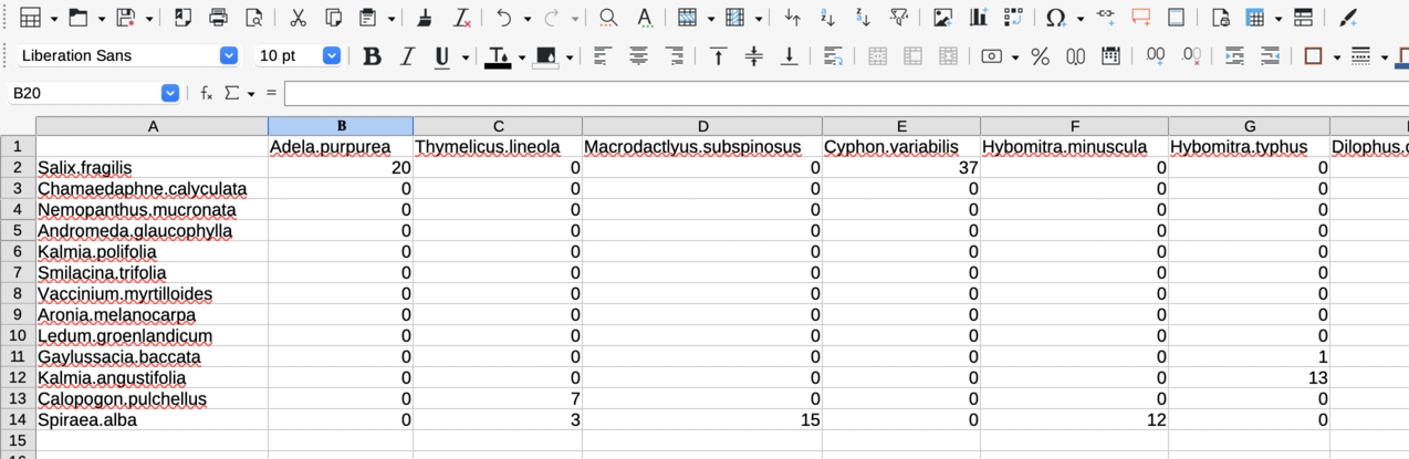
This screenshot is from LibreOffice Calc, and writes names with a “.” as separator between genus and epithet. That is a matter of taste (and actually, I do not like it).
After saving as .csv, we read this file in as:
> small1976 <- read.csv("small1976.csv", row.names=1)The row.names-argument ensures that the names in the first column are used as (row) labels in the data set. Note that this object is a data.frame, not a matrix, even though it contains only numbers. bipartite internally converts it into a matrix if that is the required format for a function.
If we want to have nicer name layouts, with an empty space instead of the ugly point, we can change it like this:
> rownames(small1976) <- gsub(".", " ", rownames(small1976), fixed=T)> colnames(small1976) <- gsub(".", " ", colnames(small1976), fixed=T)> small1976[1:5, 1:2] # to save space
Adela purpurea Thymelicus lineolaSalix fragilis 20 0Chamaedaphne calyculata 0 0Nemopanthus mucronata 0 0Andromeda glaucophylla 0 0Kalmia polifolia 0 0
This object is now in the correct format for further analysis and plotting with bipartite.
3.2 From long format in a spreadsheet to ready-for-analysis for bipartite
Raw data often start as tables of individual observations, e.g. one column containing the name of the species in the first level, another column the name of the species in the other level with which it interacts. A third column records the number of interactions for this pair, i.e. an “edge weight”:
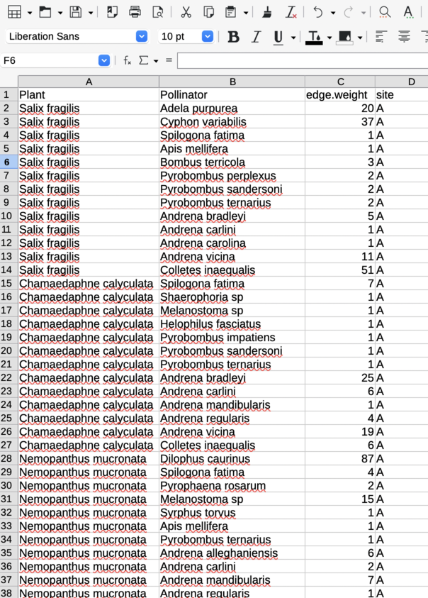
Also, several networks may be included in this table, so another column would provide a web-ID (e.g. a name of the site or the web itself). The function frame2webs is a convenience function to convert such tables into one or more webs. Its output is a list or an array of webs in the appropriate format for further analysis.33 3 webs2array can also make an array of previously separate webs, padding non-overlapping species with zeros.
> library(bipartite)> small.long <- read.csv("small1976long.csv")> small.wide <- frame2webs(small.long, varnames=c("Plant", "Pollinator", "site", "edge.weight"))> str(small.wide)
List of 1 $ A: num [1:13, 1:34] 0 0 0 0 0 0 0 0 0 20 ... ..- attr(*, "dimnames")=List of 2 .. ..$ Plant : chr [1:13] "Andromeda glaucophylla" "Aronia melanocarpa"".. .. ..$ Pollinator: chr [1:34] "Adela purpurea" "Andrena alleghaniensis" "An"..
> small.wide[[1]][, 1:2] # to save space
PollinatorPlant Adela purpurea Andrena alleghaniensis Andromeda glaucophylla 0 0 Aronia melanocarpa 0 3 Calopogon pulchellus 0 0 Chamaedaphne calyculata 0 0 Gaylussacia baccata 0 0 Kalmia angustifolia 0 0 Kalmia polifolia 0 0 Ledum groenlandicum 0 2 Nemopanthus mucronata 0 6 Salix fragilis 20 0 Smilacina trifolia 0 0 Spiraea alba 0 0 Vaccinium myrtilloides 0 0
As we see, this returns a list of networks, even if only site was provided. We can access this element using double brackets “[[1]]”. We now are back to our wide format, as required for most bipartite analyses.
3.3 From web to edge list
Many other packages (in R or otherwise) are based on one-mode representations of networks. The typical input file would be the edge list of the previous section. The function web2edges transforms bipartite “webs” into edge lists to be used e.g. in Pajek or by sna or tnet.
> head(web2edges(small1976)) # to save space
row col edge.weightsSalix fragilis 1 14 20Calopogon pulchellus 12 15 7Spiraea alba 13 15 3Spiraea alba 13 16 15Salix fragilis 1 17 37Spiraea alba 13 18 12Note that this format is different to the edge list used as input above. That is because often not the names but the positions are used as reference. That is, the numbers refers to the position in a vector {lower level species, higher level species}. In this specific case, the first pollinator species is number 14, as there are 13 plant species. Note that the row names only list the plant species: it is this plant that is visited by pollinator 14. To get the full list of names, we can simply append row and column names:
> head(c(rownames(small1976), colnames(small1976)), 16)
[1] "Salix fragilis" "Chamaedaphne calyculata" [3] "Nemopanthus mucronata" "Andromeda glaucophylla" [5] "Kalmia polifolia" "Smilacina trifolia" [7] "Vaccinium myrtilloides" "Aronia melanocarpa" [9] "Ledum groenlandicum" "Gaylussacia baccata"[11] "Kalmia angustifolia" "Calopogon pulchellus"[13] "Spiraea alba" "Adela purpurea"[15] "Thymelicus lineola" "Macrodactlyus subspinosus"
4 Visualising bipartite networks
A useful first step in the analysis of bipartite networks is to plot it. To do so, bipartite offers two main functions, plotweb and visweb. They produce a bipartite graph (e.g. Fig. 1 top) and a prettified version of the adjacency matrix (Fig. 1 bottom), respectively (Motten, 1982). Both offer a wide range of options to change sizes, colours and placement of labels. Please run example code for these functions to get a feeling for their abilities (and hopefully you’re impressed).44 4 The additional function plotweb2 is still a bit experimental but allows to combine several bipartite plots into a stack of tripartite, quadripartite, pentapartite etc. graphs. See the examples in the function’s help page for illustration. For a more in-depth guide on how to use the ploweb function also have a look at the PlottingWithBipartite vignette.
> plotweb(motten1982, srt= 90, sorting = "ca")> visweb(motten1982)
If these options are still not sufficient, and you want more customisation, such as side-by-side plotting of several networks, please check out the bipartiteD3, which provides the power of the ‘‘D3’’ library of JavaScript.55 5 The package explicitly links to “our” bipartite, although I think it is largely independent of it, and actually very nice! Note that D3 makes interactive figures, so on mouse-over the figures change. While not a feature useful for publication in the current standard, it adds 21st century appeal to such graphs.
The function plotPAC visualises (Fig. 2) a very special idea: the potential for apparent competition (Morris et al., 2005). The idea is that every parasitoid emerging from a host can attack another species. Thus, the more individuals emerge from a host, the larger is the potential for these to reduce the competition between hosts, as long as they choose their prey equiprobable. Pretty as it may be, its current value is highest for host-parasitoid networks, so the plot employing a pollination network is for illustration only.
> plotPAC(PAC(motten1982), outby=0.9)
We can also visualise communities within the network by computing its modularity and then plotting the result, using the functions computeModules and plotModuleWeb, respectively (Fig. 3).
> mod <- computeModules(motten1982)> plotModuleWeb(mod)
To visualise either level separately projected into one-mode mode, we have to employ a different package, for example sna (Butts, 2013). We can do the projection on the fly, though. For networks with even a moderate number o species, such plots can become rather obtuse and uninformative (Fig. 4).
> par(mfrow=c(1,2), xpd=T)> sna::gplot(as.one.mode(motten1982, project="higher"),+ label=colnames(motten1982), gmode="graph",+ label.cex=0.6, vertex.cex=2)> sna::gplot(as.one.mode(motten1982, project="lower"),+ label=rownames(motten1982), gmode="graph",+ label.cex=0.6, vertex.cex=2, vertex.col="green")
5 Computing indices
Network indices are primarily that: metrics to quantify an aspect of the network. Each may have a justification, a purpose, but the information in a matrix is only finite. As a consequence, network indices are highly correlated. There is thus no point in computing all indices in the book; rather should we consider very carefully what we want to test with the data and select one (or a few) indices to do so.
The bipartite-package offers itself to data dredging: with one function one can compute dozens of indices, certainly some of them will be significantly correlated with whatever we want to test. While analyses are commonly carried out in this way, this is obviously statistically inappropriate. Two issues are important here. One is that of multiple testing, and there are dozens of publications covering this issue. The other is an attempt to formalise one’s expectation. Null models are one way to do so, in particular one’s expectation of what a pattern is like in the absence of a process. This technical details of this topic are covered further below (section 6.3).
Indices (currently) come at the following hierarchical levels:
- 1.
network-level (a single value, per index, for the entire network);
- 2.
group-level (a value, per index, for each of the two groups);
- 3.
link-level (a value, per index, for each edge = link); and
- 4.
species-level (= node-level) (a value, per index, for each species).
5.1 Network-level indices
This set of indices is computed for the entire network. They are called using the function networklevel, which additionally (and conveniently) makes available all indices from the group level, too. Those restricted to the network-level are:
- 1.
connectance, also called ‘standardised number of species combinations’ in biogeographic analyses (Gotelli and Graves, 1996; Dunne et al., 2002);
- 2.
web asymmetry, the balance of the number of species in the two levels (Blüthgen et al., 2007);
- 3.
links per species;
- 4.
number of compartments;
- 5.
compartment diversity (Tylianakis et al., 2007);
- 6.
cluster coefficient, which will compute both the network-wide binary, one-mode-based cluster coefficient as well as those for each level,
- 7.
nestedness, with the returned value indicating the ‘temperature’ of the matrix, which is low () for a perfectly nested matrix (Rodríguez-Gironés and Santamaría, 2006);
- 8.
NODF, as an alternative measure of quantitative nestedness, automatically correcting for matrix filling and also indicating nestedness by values towards (Almeida-Neto et al., 2008);
- 9.
weighted nestedness, or more specifically ‘weighted interaction nestedness estimator’ (WINE), with indicating perfected nestedness (thus exactly opposite to the previous index) (Galeano et al., 2009);
- 10.
weighted NODF, as an alternative measure of quantitative nestedness, automatically correcting for matrix filling and also indicating nestedness by values towards (Almeida-Neto and Ulrich, 2011);
- 11.
interaction strength asymmetry (Blüthgen et al., 2007) (Bascompte et al., 2003, or alternatively ISA or dependence asymmetry:), which quantify whether specialised species interact with generalised ones in the other level (or vice versa);
- 12.
specialisation asymmetry (or alternatively SA), following the same idea as the previous, but this being based on species specialisation in ;
- 13.
linkage density, marginal totals-weighted diversity of interactions per species (Bersier et al., 2002);
- 14.
Fisher alpha, diversity index based on fitting a Fisher-series (Fisher et al., 1943);
- 15.
interaction evenness quantifies how balanced the distribution of interactions is across species, based on Shannon’s diversity (Tylianakis et al., 2007);
- 16.
Alatalo interaction evenness, as an alternative measure of interaction evenness, attempting to overcome some of the shortcomings of the previous, Shannon’s, version (Alatalo, 1981; Müller et al., 1999);
- 17.
Shannon diversity;
- 18.
H2, network-wide specialisation index (Blüthgen et al., 2006).
Similarly to the previous sets of indices, several options are available to fine-tune those in networklevel:
> networklevel(bezerra2009, index=c("ISA", "weighted NODF", "Fisher alpha"),+ SAmethod="log")
weighted NODF interaction strength asymmetry 5.717160e+01 8.842823e-05 Fisher alpha 8.793401e+00
5.2 Group-level indices
Indices that can be computed for each group separately are collected in the function grouplevel.66 6 If network-level indices are also desired, all indices in grouplevel are also accessible through networklevel, see below. Quite a few of these indices are aggregates from the species level (e.g. by averaging species’ degrees), in which case the mean is weighted by the number of observations of each species, thus giving more weight to species for which information is more reliable.77 7 The weighting can be switched off by stating weighted=FALSE. Others are biogeographic indices which change their value when the matrix is inverted (i.e. when a group changes from “species” to “islands”). The following indices are implemented:
- 1.
number of species in the respective trophic level;
- 2.
mean number of links;
- 3.
mean number of shared partners (Roberts and Stone, 1990; Stone and Roberts, 1992);
- 4.
cluster coefficient, which supposedly informs us whether a network has ‘small world’ properties (Watts and Strogatz, 1998);
- 5.
weighted cluster coefficient, which takes into account the number of interactions and is a properly derived bipartite version of the previous one-mode cluster coefficent above (Opsahl, 2010);
- 6.
togetherness as the mean number of co-occurrences across all pairwise species combinations (Stone and Roberts, 1992);
- 7.
C score, or ‘checkerboardness’, which averages the number of instances of 01/10-patterns (i.e. exclusive occurrences) for all pairwise species combinations (Stone and Roberts, 1990);
- 8.
V ratio, the variance ratio of species numbers to interaction numbers within species of a level (Schluter, 1984);
- 9.
discrepancy, the number of links one would have to move to achieve perfect nestedness (Brualdi and Sanderson, 1999);
- 10.
degree distribution, fitting an exponential function and (truncated) power laws(Jordano et al., 2003);
- 11.
extinction slope, with different options for the extinction sequence (Memmott et al., 2004);
- 12.
robustness, the area under the extinction curve (Burgos et al., 2007);
- 13.
niche overlap, with options for distance metrics (Pielou, 1972; Hurlbert, 1978);
- 14.
generality (for the higher trophic level) or vulnerability (for the lower one) (Bersier et al., 2002);
- 15.
partner diversity, simply the mean Shannon diversity of interactions of each species in a level;
- 16.
effective partners as before, but as the exponent of the base to which Shannon was computed (typically or ) (Jost, 2006);
- 17.
fd (or alternatively functional diversity), which is similar to niche overlap but computed as branch length of a cluster diagram of dissimilarity of resource use (Devoto et al., 2012).
As in the case of species-level indices, some allow for normalisation (between 0 and 1), others for different basis to the logarithm or similar tuning. A typical call to grouplevel will thus comprise the list of desired indices88 8 Or alternatively the argument index="ALL". and their options, as well as the level(s) for which the computation shall be carried out:
> grouplevel(bezerra2009, level="both", index=c("mean number of links", "weighted+ cluster coefficient", "effective partners", "niche overlap"), dist="bray")
mean.number.of.links.HL mean.number.of.links.LL niche.overlap.HL 9.9502551 7.0975057 0.2824538 niche.overlap.LL generality.HL vulnerability.LL 0.4795595 8.0590841 5.6963672The LL and HL behind each index indicate that it was computed for the lower and higher level, respectively. A relatively comprehensive comparison of network-level indices (Dormann et al., 2009), including some at the group level, has shown substantial redundancy among these indices, and few of them have a sound theoretical basis.
5.3 Link-level indices
At the moment, only few indices have been investigated at the level of the individual link (i.e. the cell of a network matrix):
- 1.
dependence (Bascompte et al., 2006, i.e. the relevance of each species for the other level:) one matrix for each level;
- 2.
endpoint degree (Barrat et al., 2004, i.e. product of degrees of species linked by this cell:).
It is employed by simply applying it to the network under consideration and selecting the index desired:
> str(linklevel(bezerra2009, index=c("dependence", "endpoint")))
List of 3 $ HL dependence: num [1:13, 1:13] 0.193 0.131 0.056 0.108 0.105 ... ..- attr(*, "dimnames")=List of 2 .. ..$ : chr [1:13] "Diplopterys.pubipetala" "Byrsonima.gardnerana" "Banist".. .. ..$ : chr [1:13] "Centris.aenea" "Centris.fuscata" "Centris.caxiensis" "".. $ LL dependence: num [1:13, 1:13] 0.2415 0.2238 0.0997 0.2474 0.2632 ... ..- attr(*, "dimnames")=List of 2 .. ..$ : chr [1:13] "Diplopterys.pubipetala" "Byrsonima.gardnerana" "Banist".. .. ..$ : chr [1:13] "Centris.aenea" "Centris.fuscata" "Centris.caxiensis" "".. $ endpoint : num [1:13, 1:13] 117 78 156 104 91 65 52 26 52 52 ... ..- attr(*, "dimnames")=List of 2 .. ..$ : chr [1:13] "Diplopterys.pubipetala" "Byrsonima.gardnerana" "Banist".. .. ..$ : chr [1:13] "Centris.aenea" "Centris.fuscata" "Centris.caxiensis" ""..This function is so rudimentary, and its output so disproportionally voluminous, that it is not worth going into further details here and use str to only show the structure of the output.
5.4 Species-level (= node-level) indices
The (growing) list of indices computable for each species in the network comprises (the index name to be used in the call is given in typewriter font):
- 1.
degree, i.e. the number of links of each species,
- 2.
normalised degree for a normalised version of degree (Martín González et al., 2010),
- 3.
species strength as sum of dependencies for each species (Bascompte et al., 2006),
- 4.
nestedrank as rank in a nested matrix (Alarcón et al., 2008),
- 5.
interaction for interaction push/pull (a version of dependence asymmetry), (Vázquez et al., 2007),
- 6.
PDI for Paired Differences Index (Poisot et al., 2011b; Poisot et al., 2011a),
- 7.
resource range for Schoener’s index of unused resources (Schoener, 1989),
- 8.
species specificity (or coefficient of variation of interactions) (Julliard et al., 2006; Poisot et al., 2012),
- 9.
PSI for pollination service index (or pollinator support index, depending on the trophic level),99 9 devised by the author with Nico Blüthgen and Bernd Gruber
- 10.
NS for node specialisation index (Dalsgaard et al., 2008),
- 11.
betweenness for betweenness (Borgatti and Everett, 1997),
- 12.
closeness (both automatically also return their weighted counterparts proposed by Tore Opsahl in package tnet),
- 13.
Fisher for Fisher’s alpha as a measure of diversity (Fisher et al., 1943),
- 14.
diversity for Shannon diversity of interactions of that species,
- 15.
effective partners for the effective number of interacting partners (Bersier et al., 2002),
- 16.
proportional generality for a quantitative version of normalised degree,1010 10 devised by Jochen Fründ
- 17.
proportional similarity as specialisation measured as similarity between use and availability (Feinsinger et al., 1981),
- 18.
d for Blüthgen’s discrimination/selectivity index (Blüthgen et al., 2006).
Some of them allow for normalisation (between 0 and 1), others for different basis to the logarithm or similar tuning. A typical call to specieslevel will thus comprise the list of desired indices1111 11 Or alternatively the argument index="ALL". and their options, as well as the level(s) for which the computation shall be carried out:
> specieslevel(bezerra2009, level="lower", index=c("normalised degree", "PDI",+ "effective partners"), PDI.normalise=F)
normalised.degree PDI effective.partnersDiplopterys.pubipetala 0.6923077 1010.0000 7.437631Byrsonima.gardnerana 0.4615385 1939.6667 3.819660Banisteriopsis.muricata 0.9230769 657.0000 9.191488Heteropterys.sp1 0.6153846 570.3333 6.278285Heteropterys.sp2 0.5384615 567.3333 5.865968Dicella.bracteosa 0.3846154 429.0000 4.582040Carolus.chasei 0.3076923 513.6667 3.751208Stigmaphyllon.paralias 0.1538462 774.0000 1.944388Banisteriopsis.stellaris 0.3076923 245.6667 3.787887Banisteriopsis.schizoptera 0.3076923 189.0000 3.822392Stigmaphyllon.auriculatum 0.3076923 204.3333 3.687447Stigmaphyllon.ciliatum 0.2307692 238.0000 2.937197Janusia.anisandra 0.2307692 220.3333 2.813322A relatively comprehensive comparison of species-level indices of specialisation, Dormann (2011) has shown substantial redundancy among these indices, and only few of them have a sound theoretical basis (Poisot et al., 2012).
5.5 Which index to choose?
Different indices were invented (“developed”) for different purposes. However, for most indices, it has not been demonstrated that they actually achieve what their inventor had in mind. Most commonly indices quantify a specific pattern which may have come about by a whole variety of different causes. Take, for example, connectance, i.e. the proportion of possible links actually recorded. Low connectance may be caused by high specialisation or by low sampling intensity. The same holds true for a species’ degree, which (typically) increases with sampling effort as well as generalisation. For the choice of an index this means that we cannot solely rely on what the inventor has proposed this index to be good for, but we have to keep in mind that it may actually quantify several other things, too.
Apart from the different levels at which an index can quantify a network pattern (from the individual link to the entire network, as covered in sections 5.3–5.1), indices can be divided into those for binary and those for weighted data (called here binary and weighted indices, respectively). Binary indices only use the information of whether a link exists, while weighted indices additionally account for how strong a link is, as judged from the actual value in a network matrix.
Binary indices, by definition, use less information. It does not follow that they are thus more robust! In fact, Blüthgen (2010) argues the opposite, since only a weighted index can tell whether an observed value indicates specialisation or not.1212 12 Imagine two species, one with entries (1, 1), the other with entries (1, 100). A binary index would not be able to tell between them, while a quantitative would expose the second as far more specialised.
This, if two indices are available to quantify the same idea, one binary and one quantitative, one should generally choose the quantitative one. Rather than species degree, we should use species strength or linkage density. Table 1 depicts some such binary-quantitative index pairs.
| binary | quantitative | |
|---|---|---|
| network level | connectance | |
| links per species | linkage density | |
| nestedness | weighted NODF, wine | |
| group level | mean number of partners | effective number of partners |
| species level | degree | species strength, effective number of partners |
In a nutshell: Quantitative indices make use of more information in the data. They are generally more advisable, although most of them also are strongly affected by sampling issues.
5.5.1 One index, many values: A cautionary tale told by the betweenness mess
Betweenness is a graph index which quantifies the importance of a node for fluxes between nodes. It does so by counting how many of all shortest paths between two nodes go through the target node. That means, a peripheral node will have a betweenness score of 0, while a central node can have values up to (if all shortest paths go through it).
> data(Safariland)> # plot the one-mode projection for the lower level:> set.seed(4) # don't ask me why gplot is stochastic ...> par(xpd=T, mar=c(0,6,0,6))> sna::gplot(as.one.mode(Safariland, project="lower"), label=rownames(Safariland))
So, what we see is for the main module a rather central position for, e.g., Rosa eglanteria. For 8 species (we can neglect Cynanchum diemii), we have paths. For a simple example, Aristotelia chilensis (plant number 1 in the edge list below) should have only the shortest path to Schinus patagonicus running through it, to all other 6 plant species.
Let’s see what its betweenness score is, using several different functions across R-packages:
> # convert matrix into one-mode edgelist:> SafPlantsEL <- as.tnet(as.one.mode(Safariland, project="lower"))
> # compute betweenness:> tnet::betweenness_w(SafPlantsEL) # 6> bipartite::BC(Safariland, rescale=F)$lower # 6> DiagrammeR::get_betweenness(DiagrammeR::from_igraph(tnet_igraph(SafPlantsEL))) # 6> igraph::betweenness(tnet_igraph(SafPlantsEL), cutoff=9) # 6> influenceR::betweenness(tnet_igraph(SafPlantsEL)) # 12> sna::betweenness(SafPlantsEL) # length 36!!> sna::betweenness(as.matrix(SafPlantsEL)) # length 27!!
Let’s put them all next to each other, into a named matrix:
> btws <- cbind("t:betw"=tnet::betweenness_w(SafPlantsEL)[,2],+ "b:BC"=bipartite::BC(Safariland, rescale=F)$lower,+ "DR:betw"=DiagrammeR::get_betweenness(DiagrammeR::from_igraph(tnet_igraph(SafPlantsEL)))[,2],+ "i:estbetw"=igraph::betweenness(tnet_igraph(SafPlantsEL), cutoff=9),+ "inf:betw"=influenceR::betweenness(tnet_igraph(SafPlantsEL))/2 )> rownames(btws) <- rownames(Safariland)> btws
##                          t:betw b:BC DR:betw i:estbetw inf:betw
## Aristotelia chilensis         6    6       6         6        6
## Alstroemeria aurea           11   10      14        14       10
## Schinus patagonicus           0    0       0         0        0
## Berberis darwinii             0    0       0         0        0
## Rosa eglanteria              13    4       6         6        4
## Cynanchum diemii              0    0       0         0        0
## Ribes magellanicum            0    0       0         0        0
## Mutisia decurrens             0    0       0         0        0
## Calceolaria crenatiflora      0    0       9         9        0
So they all agree on the betweenness-value for Aristotelia, but not for Alstroemeria and Rosa, and not at all for Calceolaria.
The case of Calceolaria is instructive. Here we can see that actually none of the shortest paths goes through its node, making a value of 9 incorrect. (Try finding a single path that cannot be short-cutted through a link between Alstroemeria.)
Also Rosa is instructive. Here we encounter the problem of ties: several shortest paths are on equal footing, e.g. Aristotelia - Rosa - Ribes is as short as Aristotelia - Alstroemeria - Ribes. In fact, there are 4 unique shortest paths through Rosa, but 6 shortest paths in total. So it seems that DiagrammeR and igraph simply handle ties differently to bipartite’s BC and influenceR. Tnet’s betweenness_w1313 13 Available in bipartite under the same name. remains a mystery. Even if 13 may be the number of all paths, then that would not explain the many 0s for the other species.
Note that all functions used here have options and arguments that affect the outcome. Setting them differently will yield, for example, standardised values. We only investigated out-of-the-box behaviour and are not suggesting something is actually wrong with the functions, but you may have to tweak them to yield an intuitive result. A case in point is influenceR’s betweenness, which will return igraph’s value if the argument snap is set to FALSE, but 2*BC’s values for the default (TRUE).
To summarize: bipartite::BC and influenceR::betweenness/2 yield values as one would expect for unique shortest paths; DiagrammeR::get_betweenness and igraph::betweeness yield number of non-unique shortest paths, which we also regard as an intuitive measure.
As always in data analysis: it is the responsibility of the analyst to make sure suitable-for-purpose indices are used!
5.5.2 Index redundancy: do different indices tell the same thing?
To visualise the similarity and possible redundancy of the different indices, they are computed for the networks in bipartite and summarised through a principal component analysis (see Fig. 5).
> web.names <- data(package="bipartite")$results[,3]> data(list=web.names) #loads all webs> # the next step takes around 10 minutes:> netw.indic.webs <- t(sapply(web.names, function(x) networklevel(get(x),+ index="ALLBUTDD")))
> PCA.out <- prcomp(netw.indic.webs[,-5], scale.=T)> biplot(PCA.out, xpd=T, las=1)
> summary(PCA.out)
Importance of components: PC1 PC2 PC3 PC4 PC5 PC6 PC7Standard deviation 4.2780 3.6461 2.09732 1.84163 1.32612 1.09350 1.0375Proportion of Variance 0.3979 0.2890 0.09562 0.07373 0.03823 0.02599 0.0234Cumulative Proportion 0.3979 0.6869 0.78248 0.85621 0.89444 0.92044 0.9438 PC8 PC9 PC10 PC11 PC12 PC13 PC14Standard deviation 0.81058 0.64158 0.62560 0.56960 0.49217 0.43179 0.36230Proportion of Variance 0.01428 0.00895 0.00851 0.00705 0.00527 0.00405 0.00285Cumulative Proportion 0.95812 0.96707 0.97558 0.98263 0.98789 0.99195 0.99480 PC15 PC16 PC17 PC18 PC19 PC20 PC21Standard deviation 0.26591 0.25249 0.2254 0.18080 0.11401 0.09049 7.038e-16Proportion of Variance 0.00154 0.00139 0.0011 0.00071 0.00028 0.00018 0.000e+00Cumulative Proportion 0.99634 0.99772 0.9988 0.99954 0.99982 1.00000 1.000e+00
Apparently 40, 30 and 10% of the variation in indices can be partitioned to the first three axes. We can now investigate which indices load on the few axes:
> round(PCA.out$rotation[, 1:4], 3)
PC1 PC2 PC3 PC4connectance 0.177 0.147 -0.044 0.025web asymmetry -0.137 -0.098 -0.298 0.063links per species 0.189 -0.087 -0.020 0.183number of compartments -0.147 0.005 0.167 -0.051cluster coefficient 0.169 0.128 0.005 0.119nestedness -0.020 0.196 -0.004 0.305weighted nestedness 0.066 -0.108 -0.170 -0.399weighted NODF 0.193 0.068 -0.138 -0.182interaction strength asymmetry -0.172 0.080 -0.178 -0.028specialisation asymmetry 0.021 0.109 0.337 -0.096linkage density 0.049 -0.258 -0.058 -0.038Fisher alpha -0.041 -0.246 0.045 -0.053Shannon diversity 0.073 -0.251 0.011 0.082interaction evenness 0.179 -0.078 0.012 0.102Alatalo interaction evenness 0.076 0.159 0.143 -0.045H2 -0.191 0.089 0.091 0.037number.of.species.HL -0.048 -0.249 0.026 -0.062number.of.species.LL -0.020 -0.256 0.121 -0.038mean.number.of.partners.shared.in.HL 0.191 -0.032 -0.177 0.189mean.number.of.partners.shared.in.LL 0.218 0.042 -0.049 -0.042cluster.coefficient.HL 0.189 0.093 -0.001 -0.036cluster.coefficient.LL 0.155 0.085 -0.285 -0.009weighted.cluster.coefficient.HL 0.150 -0.122 -0.189 0.162weighted.cluster.coefficient.LL 0.212 -0.040 0.035 0.145niche.overlap.HL 0.045 0.142 -0.287 -0.272niche.overlap.LL 0.202 0.035 0.062 -0.195togetherness.HL 0.023 0.181 -0.283 -0.032togetherness.LL 0.216 0.052 0.087 -0.041C.score.HL -0.162 -0.123 0.217 0.147C.score.LL -0.216 -0.020 0.038 0.026V.ratio.HL 0.177 -0.121 0.121 -0.101V.ratio.LL -0.048 -0.238 -0.151 -0.113discrepancy.HL -0.041 -0.251 0.059 -0.042discrepancy.LL -0.039 -0.252 0.062 -0.037extinction.slope.HL 0.216 -0.006 0.063 0.131extinction.slope.LL 0.120 -0.061 0.035 0.326robustness.HL 0.214 -0.020 0.059 0.148robustness.LL 0.150 -0.084 -0.114 0.254functional.diversity.HL 0.162 0.003 0.027 -0.257functional.diversity.LL 0.163 -0.003 0.029 -0.259partner.diversity.HL 0.198 -0.078 0.183 -0.028partner.diversity.LL 0.061 -0.222 -0.212 0.082effective.partners.HL 0.187 -0.079 0.206 -0.101effective.partners.LL -0.003 -0.256 -0.125 -0.011generality.HL 0.187 -0.079 0.206 -0.101vulnerability.LL -0.003 -0.256 -0.125 -0.011As we can see, there are quite a few indices on the first axis with a loading of around 0.2 (links per species, weighted NODF, H2, mean number of partners shared; weighted cluster coefficient, niche overlap, togetherness, C-score (all lower level); extinction slope, robustness, partner diversity (all higher level)).
Also the PCA biplot (Fig. 5) is not very helpful, since the many indices pointing “southwards” are unreadably overlapping.
Alternatively, we might want to depict the correlation between different indices by means of a cluster analysis (Fig. 6).
> library(Hmisc)> plot(varclus(netw.indic.webs), cex=0.8)> abline(h=0.5, lty=2, col="grey")
It picks out a slightly different structure, with the PC1 being distributed over more than one cluster (towards the left, with extinction.slope.HL but also towards the centre, with weighted NODF). In either case it becomes clear that many indices are of limited originality. However, there are some branches ending above the dashed line, indicating that they add a new element to the description of the network. Some are trivial, such as the number of species in the lower level, others less so (specialisation asymmetry, extinction slope LL, niche overlap HL, (weighted) nestedness).
It should become clear that there is no need to compute all indices a software can offer, and that some clusters seem to measure the same latent property, even it is unclear what that property is. Curiously, higher and lower level indices are always intermixed. There seems to be always an effect onto the other level, so that some indices pick up a signal in one level, but others the same signal in the other.1414 14 That should be the case for extinction slopes and robustness, which measures the response of one level to extinctions in the other. But is difficult to see why the cluster coefficient for the higher level should be correlated with togetherness in the lower. Post hoc, it is always possible to find a reason, but a priori this is not expected.
The 22 pollination networks, on which both PCA and cluster are based, are most certainly not representative of bipartite networks in general. The simulations of Dormann et al. (2009) for a wider range of sizes and linkage densities show a qualitatively similar picture, though: indices are overlapping into clusters.1515 15 We could similarly say that there is a substantial redundancy in network indices, evident from the analysis where we condense 92% of variation in 40 odd indices onto six axes.
5.5.3 Variations on on the same theme: which index of a group of similar ones should I choose?
Different indices were developed for different aims. Some are very reasonable, logically sound, thoughtful and even productive (in the sense of “shown to be doing what they are supposed to do”), others aren’t. Each index should be understood when being used, based on the literature introducing it and any later study refining, comparing or criticising/appraising it. There is no easy way to decide the question “Which is the right index for me?”
That said, there are a few guiding considerations that seem plausible to me:
- 1.
Quantitative indices use more information than binary ones; preferably use the former.
- 2.
Indices developed for bipartite networks are likely to be closer, theoretically, to the structure of the data than one-mode indices working on projections of bipartite networks.
- 3.
Indices that came out positively in comparisons have proven their worth more than fresh-off-the-press indices.
- 4.
If two or more indices seem barely distinguishable, do not choose the one easiest to interpret! This would be a logical fault, since their similarity indicates clearly that they are affected by “something” and we don’t know what that something is, yet. But interpreting an effect as being caused by what is “most convenient to interpret” is most certainly wrong (Shermer, 2012).1616 16 Of the many, many biases that can creep into scientific explorations, this is one. We could call it the “parsimony bias” as a special case of the “selection bias” (Shermer, 2012).
The last point in particular seems rather little helpful. Imagine the two index values “functional diversity” for the higher and lower trophic level, which are near-identical in Fig. 6. This indicates that the network, rather than each level, contains the information which these two indices describe. In this particular case, we may want to consider using neither index, or using any of them but interpreting it as if it represented both level.
Thus, in a nutshell, there is no easy answer and there is no way around knowing the index and the literature about it and its friends.
6 Null models
6.1 Why null models?
When a network is structured according to some measure (e.g. nestedness), what does that mean? It could mean that ecological processes leading to nestedness are at play. Or it could mean that a sampling effect makes nestedness an inevitable consequence. Or, finally, it could be a mixture of both. Furthering our understanding of nature is not aided by the reporting of spurious relationships resulting from sampling effects, hence a formal description of what the network would look like without the ecological process would be a useful comparison. That is what a null model aims to provide (Gotelli and Graves, 1996).
In ecology, null models are common only in some fields, particularly in biogeography (Gotelli and Graves, 1996; Hausdorf and Hennig, 2007), but also in network analyses (Dormann et al., 2009; Joppa et al., 2009; Blüthgen et al., 2008; Vázquez and Aizen, 2006; Vázquez and Aizen, 2003; Vázquez et al., 2009). With respect to particular bipartite indices, some studies rejected the current nestedness paradigm using abundance-based null models, for observed (Kallimanis et al., 2009; Moore and Swihart, 2007; Santamaría and Rodríguez-Gironés, 2007), as well as for simulated networks (Krishna et al., 2008).
Null models extend much beyond ecology and were probably first used in physics. Latapy et al. (2008) use them to investigate degree distributions in non-ecological bipartite networks. Using another network example, the module detection algorithm proposed by Newman and Girvan (2004) also uses a null model to define a “group” (or module or community) within a network: there are more links within than between groups. The null model then is a random network with as many links between as within groups (Guimerà et al., 2005). In its quantitative version, the null model is constructed from proportionally probable interactions by differently abundant participants (Barber et al., 2004). The specific null model used above is underlying most current implementations of contingency table tests such as or Fisher’s signed rank test (Patefield, 1981).
In conclusion, null models are established approaches in physics as well as ecology to correct for statistical artefacts and to establish an expectation in the absence of the hypothesised structuring mechanism.
6.2 Justifying conservative null models
The interactions observed in a network are the result of a dynamic interaction between species at two levels. If we use null models to represent the outcome of these interactions (the abundances of the participants), we seem to be over-correcting. How can we possibly find a pattern, if we use this pattern as a null model? Is an abundance-based null model not a circular argument? Here I argue when it is not, and if circularity would sneak in, why it would still be better to over-correct. I shall focus on pollination networks, and every network analyst has to decide in how far this reasoning can be applied to his/her system.
Plant persistence in a site depends to some extend on them being pollinated, and pollinator population dynamics is affected by the amount of nectar and pollen they collect from the flowers they visit. However, plant growth and population dynamics are also affected by nutrient and light availability, save sites for seed germination, herbivory and fungal pathogens, mycorrhisation and environmental disturbances; and similar constraints exist for pollinators. It is thus difficult, if not impossible, to say how much of the observed abundance of a species (plant or pollinator) is caused by the specific plant-pollinator interaction and hence the structure of the network. To the extent that abundances are determined by the pollination interaction we may indeed introduce collinearity. To date, there are no data to estimate the proportion of population growth controlled by mutualistic interactions of either plants or pollinators. We can only guess based on observations such as strong nest-site limitation in solitary bees (Steffan-Dewenter and Schiele, 2008), relatively high parasitism rates of pollinators (Klein et al., 2002), strong nutrient limitations of plant population dynamics (Ghazoul, 2005) and grazing pressure (Crawley, 1987; de Mazancourt and Loreau, 2000) that they are probably not dominating population dynamics. On the other hand, clear (but rare) examples of co-evolution indicate that such a strong mutual dependence may indeed occur (Waser et al., 1996; Waser and Ollerton, 2006).
Secondly, the observed interactions are not necessarily reflecting abundance of flowers or pollinators, but rather their attractiveness (e.g. due to scent, colouration or nectar production) and activity (e.g. daily period of foraging, phenology through the season, temperature- dependence of foraging activity), respectively. Hence by using observed sums of observed interactions, one does not correct for abundance, but for attractiveness and activity, respectively.
Third, the null model uses marginal totals, i.e. summed across all links of a species. If a pollinator was specialised on a single plant species, the null model would scatter these interactions across all and hence correctly identify a miss-match between observed and null model. If, on the other hand, a pollinator was generalised, then the scattering of interactions across all plant species would also yield a similar picture and generalisation would correctly be inferred.
Finally, even if the null model used would introduce some amount of circularity and thus “over-correction”, we have to balance this against “over-detection”. Finding specialisation in an uncorrected approach will incur high levels of type I error (i.e. detecting a pattern that is actually not there). A null model insures against this type of error. We can thus be sure that a pattern that “survives” the null model test is no statistical artefact. Since it has been shown repeatedly that sampling intensity and “natural” differences in abundance will cause such artefacts (Dormann et al., 2009; Blüthgen, 2010; Joppa et al., 2009; Blüthgen et al., 2008), they must be addressed. Ignoring them will lead to misinterpretation and over-reporting of spurious network structure. After correction for expectation based on abundances, we can start understanding ecology (Vázquez et al., 2007).
In conclusion, circularity is unlikely to substantially impair null models for pollination networks. The risk of reporting non-existent network structure and further speculation of network stability due to this spurious network structure is a problem that requires a correction, even if circularity was present.
6.3 Using null models to test for significant tests in data
Once you have settled on a null model, there are fundamentally two different approaches to use such null models in statistical significance testing: corrected indices and null modelling the entire analysis. Let us look at them in turn, starting with the seemingly easier option.
Corrected indices and -scores
Imagine we computed the index for a network. We now want to know whether this value is anything special, given the abundances of the species.1717 17 Thereby we justify the use of the Patefield algorithm as null model. But the approach is independent of which null model we use. So we build, say, 1000 null models1818 18 E.g. using nulls <- nullmodel(web=Safariland, N=1000, method=’r2d’) and compute our index for each of them. We can visualise the distribution of null-model -values relative to our observed index value (Dormann et al., 2009).
> data(Safariland)> Iobs <- nestednodf(Safariland)$statistic[3]> nulls <- nullmodel(web=Safariland, N=1000, method='r2d') # takes a while!> Inulls <- sapply(nulls, function(x) nestednodf(x)$statistic[3])> plot(density(Inulls), xlim=c(0, 100), lwd=2, main="NODF")> abline(v=Iobs, col="red", lwd=2)
All that is fine for a single network, but no option if we want to analyse dozens or hundreds of networks. We thus have to summarise this figure in a value. The simplest, most obvious but generally not best solution would be to subtract the null model mean from the observed, so that . The reason why this is not ideal is that the null model distribution is likely to vary from network to network. Thus, a difference of, say, 20 may be a lot for pointy distributed null models such as the one in Fig. 7, but only little for null model values spreading over the entire -axis.
The better, and more established approach, would be to compute -scores (= standard scores or normal scores) for each network, which express the difference in terms of standard deviations of the null distribution:
We can now analyse the -scores instead of the original -values.
-scores have one major disadvantage for several of the network indices presented earlier: the standard deviation becomes an unsuitable measure of spread as the values approach an upper or lower bound. Imagine our network index is bound between 0 and 1 (as many are). If the null models have values above, say, 0.9, the upper bound is so close that the distribution will be skewed and the standard deviation biased too low. This may lead to inflated -scores. So whenever you observe values close to either bound, beware of distorted -scores.
Null-model the entire analysis
The alternative approach is to carry out the intended analysis on the observed index values and then, in a second step, repeat it with one realisation of a null model per network. Next, repeat this second step several thousand times (for good measure) and store the statistics you are interested in (say -values in an ANOVA or slopes in a regression). Instead of using the -values from the analysis of the observed values, compare observed and null-modelled statistics and count the proportion of values exceeding the observed and use those as -value. To anyone with any experience in resampling analysis or bootstrapping this is standard procedure (Efron and Tibshirani, 1993; Manly, 1997).
As an example, we can use a question addressed in Vázquez and Simberloff (2003), where the authors investigate whether cattle grazing affects the network structure of pollination networks in four replicated sites in Argentina. As response we haphazardly choose linkage density.
> weblist <- lapply(c("Safariland", "vazarr", "vazllao", "vazcer", "vazmasc",+ "vazmasnc", "vazquec", "vazquenc"), get)> # Write a function to compute the desired statistic, e.g. the difference> # between grazed and ungrazed:> meandiff <- function(webs){+ obs <- sapply(webs, networklevel, index="linkage density")+ mean(obs[1:4]) - mean(obs[5:8])+ }> (observed <- meandiff(weblist))
[1] -0.2481145Now generate a null model and repeat:
> nulllist <- lapply(weblist, nullmodel, N=1, method="r2d")> meandiff(weblist)
[1] -0.2481145Repeat this procedure, say, 5000 times:1919 19 For didactic purposes, we use an inelegant but easy to understand for-loop here. In productive mode we would instead use sapply or replicate, which would make the code more compact, but in this case not faster.
> res <- 1:5000> for (i in 1:5000){ # takes a few minutes !!+ nulllist <- sapply(weblist, nullmodel, N=1, method="r2d")+ res[i] <- meandiff(nulllist)+ }Finally, we can depict the results in a histogram (Fig. 8), with observed as vertical line, and compute the -value based on the 5000 null models:
> hist(res, xlim=c(-0.3, 0.3), border="white", col="grey")> abline(v=observed, col="red", lwd=2)> # compute p-value as proportion smaller or than observed> sum(res < observed)/length(res) * 2 # *2 for two-tailed testThe idea here is to compute a statistic of interest, in this case the mean difference between some network index for the two treatments, and then use the null model to compute expectations. In the above example, we would apparently expect no difference (which is intuitive); additionally we also get an idea of how much variability we can expect (the distribution of the null model-based mean differences in linkage density). Thus, in this example, the difference in linkage density of pollination networks from grazed vs ungrazed pastures is highly significant ().
7 Modularity
Aggregated sets of interacting species are called ‘modules’. Their defining feature is that within-module interactions are more prevalent than between-module interactions (Newman, 2003; Newman and Girvan, 2004; Fortunato, 2010). In other words, modules are link-rich clusters of species in a community. What causes such modules and whether they actually teach us something is discussed at length by Dormann et al. (2017).
There are several algorithms for one-mode networks, particularly for binary one-mode networks, such as the Louvain algorithm, the infomap or Clauset et al. (2004)’s “fast greedy” algorithm. These algorithms vary substantially in their robustness, in the sense that small changes in the network may yield very different modules, as compared by Policastro et al. (2021). That paper also expores ways to test for significance of modularity, based on null model simulations.
The package bipartite offers an algorithm (Dormann and Strauß, 2014, QuaBiMo, described in technical detail in) to detect modules in bipartite networks, taking into account the quantitative nature of links. The algorithm has become outdated after a vastly improved approach was published by Beckett (2016), which is also now the default algorithm used in bipartite’s computeModules function.
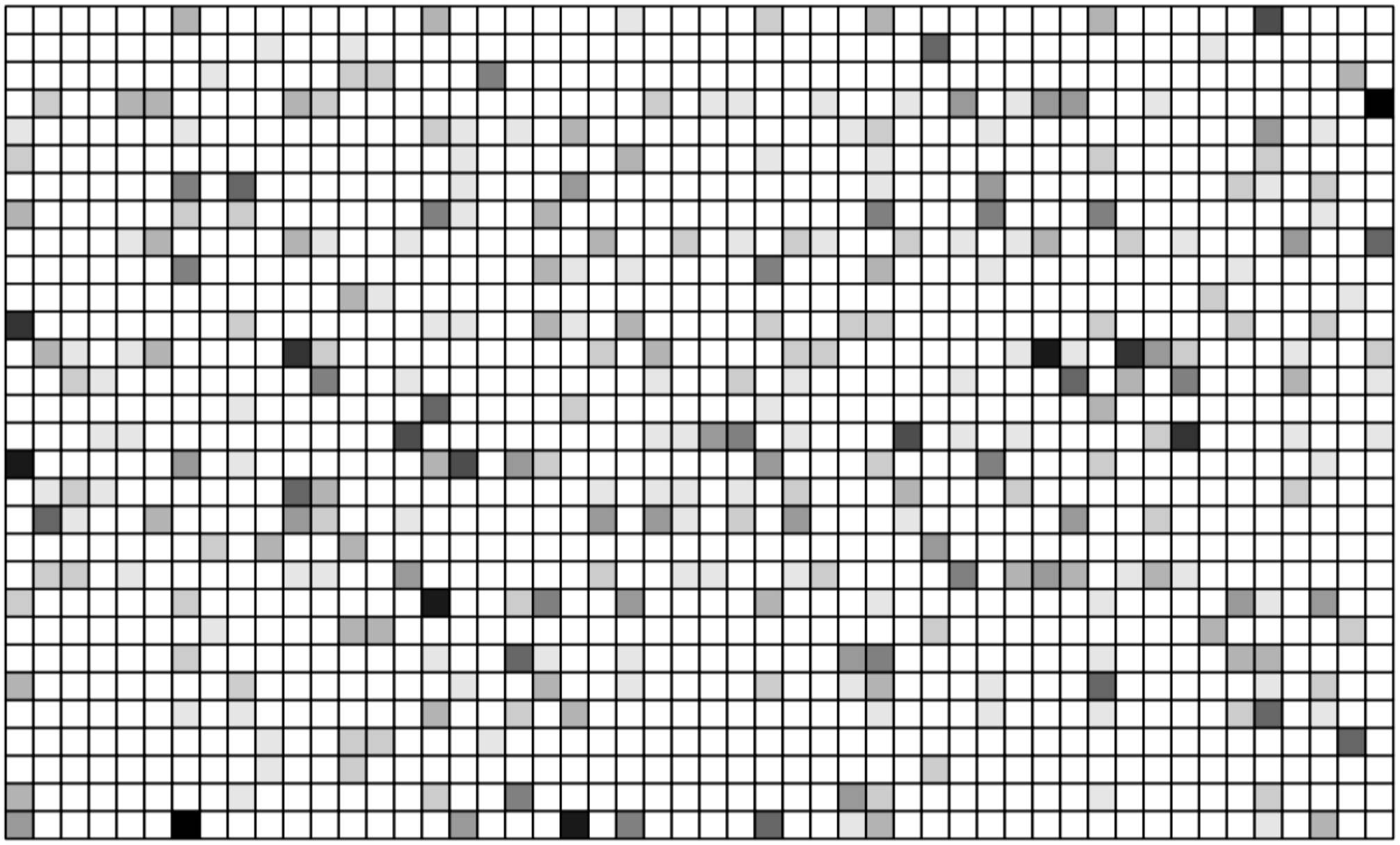
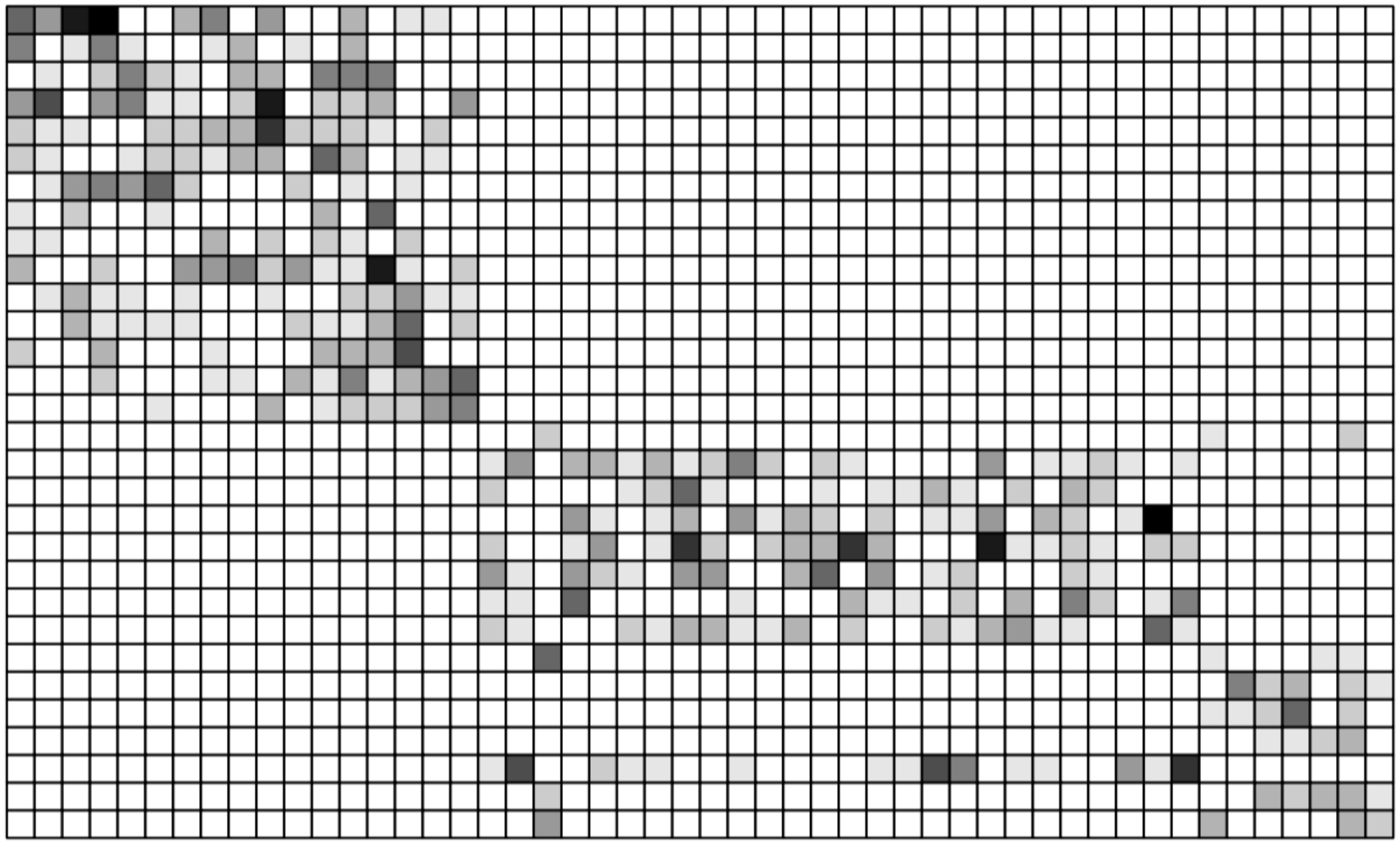
Old-school modularity was identified using correspondence analysis, which, however, will not be able to identify modules sufficiently well, even if modules are actually compartments (i.e. perfectly separated: Fig. 9 left, centre). The algorithm used in bipartite can do so, at least in principle (Fig. 9 right).2020 20 As a note on terminology: If modules are perfectly separated, with no species interacting with species in another module, they are called “compartments” and will be visible as clearly separated blocks of interacting species. It is relatively straightforward to implement a recursive compartment detection function, but compartments are too much black-and-white compared to modules and often only occur in ecological networks because sampling was rather incomplete or very different habitats were sampled.
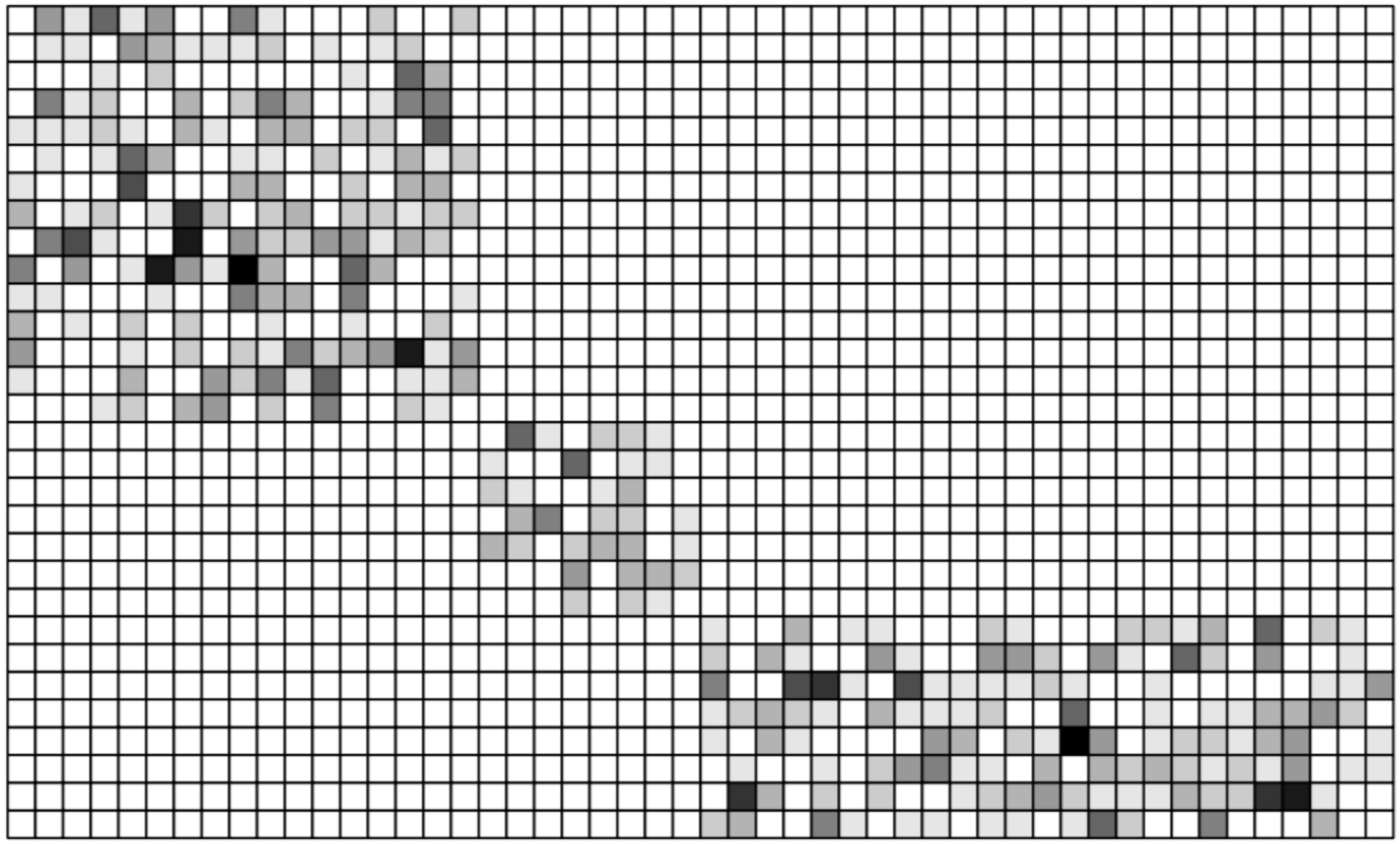
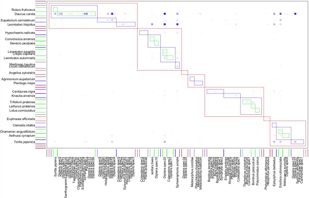
QuaBiMo can be invoked recursively (we are working on doing the same for Beckett), searching for modules within modules (Fig. 10, bottom). While such nested modules become ever smaller and are thus ever faster to detect, there are plenty of them and hence nesting will typically dramatically prolong computing time during the search for patterns (Memmott, 1999).
Modularity is likely to be correlated with other network metric, as specialisation of module members is the prime reason for the existence of modules. Across the (then) quantitative pollination networks of the NCEAS “interaction webs” data base, was evidently highly positively correlated with complementary specialisation (Fig. 11). Ecologically, the correlation with specialisation makes good sense. Modules only exist because some species do not interact with some others, i.e. because they are specialised. An overall low degree of specialisation is equivalent to random interactions, which will yield no modules.
Furthermore, the absolute value of is, like all network indices (Dormann et al., 2009), dependent on network size (i.e. the number of species) as well as the number of links and the total number of interactions observed (Thébault, 2013). We would thus recommend a null model comparison (Vázquez and Aizen, 2003; Blüthgen et al., 2008; Dormann et al., 2009) to correct the observed value of by null model expectation (e.g. by standardising them to -scores: ). Modularity is in itself not an index of an ecological feature. It is merely a measure of how well links and interactions can be separated into different modules. Large networks, with many species and links, allow for more combinations of species-in-modules, leading to higher values of , as Allesina and Pascual (2009) pointed out for any grouping algorithm.
7.1 Using modularity to identifying species with important roles in the network
Guimerà et al. (2005) and Olesen et al. (2007) propose to compute standardised connection and participation values, called and , for each species to describe their role in networks, where refers to the between-modules connectivity (Guimerà et al., 2005, called “participation coefficient” :) and refers to within-module degrees. Originally, both are computed based on the number of links, but a weighted version based on species strength is implemented, too. Guimerà et al. (2005) suggest critical values (only for the binary approach) of and of and , respectively. Species exceeding both of these values are called “hubs” because they link different modules, combining high between- with high within-module connectivity.
In the case of the pollination network of Fig. 10, -values range between and (with of pollinators and of plant species exceeding the threshold of ); -values range between and (with two pollinators but no plant species exceeding the value of : Fig. 12). Put together, only the syrphid Syritta pipiens (and hawkbit Leontodon hispidus almost) exceeded both thresholds and would thus be called a “hub species”. As can be seen in Fig. 10, this syrphid is relatively rare but clearly not randomly distributed over the six modules, thus linking three highest-level modules. In contrast, Leontodon hispidus is a common plant species, visited by many different pollinators, and it actually links almost all modules.
To objectively define this threshold one could run null models of the original network and employ % quantiles as critical - and -values. For the pollinators in the network of Fig. 10 these would be () and (), respectively, based on null models (for plants: and ; Fig. 12 left). While for plant species this has little effect (except for moving Leontodon hispidus across the threshold), three more pollinators would become hub species (the common hoverfly Episyrphus balteatus, the tachinid fly Eriothrix rufomaculata and undetermined fly “Diptera spec.22”).
8 Analyses beyond bipartite
Of course, there are many different packages that analyse one or the other aspect of networks, and some even of bipartite networks (listed in the introduction of this vignette). Some of them we find particularly interesting or useful or innovative, and here we quickly show some of them at work.
8.1 Plotting pretty bipartites
The plotting functions provided by bipartite are somewhat rudimentary. We’re happy with them, and they are surprisingly flexible already, but our graphical skills (and intentions) are limited. Other people have developed plotting functions/solutions, which we shall briefly (and probably incompletely) show here.2121 21 Partly based on this question on SO: https://stackoverflow.com/questions/31366066/how-to-plot-a-bipartite-graph-in-r
8.1.1 bipartiteD3
This package allows for very customised plotting. The coolest thing about bipartiteD3 is that it can be used interactively. By moving the mouse over the plot, the link colours change and so forth.
However, it is a bit awkward as it produces a plot in the viewer (or wherever), which then has to be saved and linked back into the document. Quite often, the plot is then incomplete, as in the example below (where the percentages are cut off despite being visible in the export-window of RStudio).
Here is a very short and simple default plot:
> library(bipartiteD3)> bipartite_D3(small1976, colouroption = 'brewer', ColourBy = 1,+ PercentageDecimals=1, filename = 'small1976Plot')After saving the resulting image, it looks like this, wth the percentages representing the proportion of links in the network of the particular node (= species).
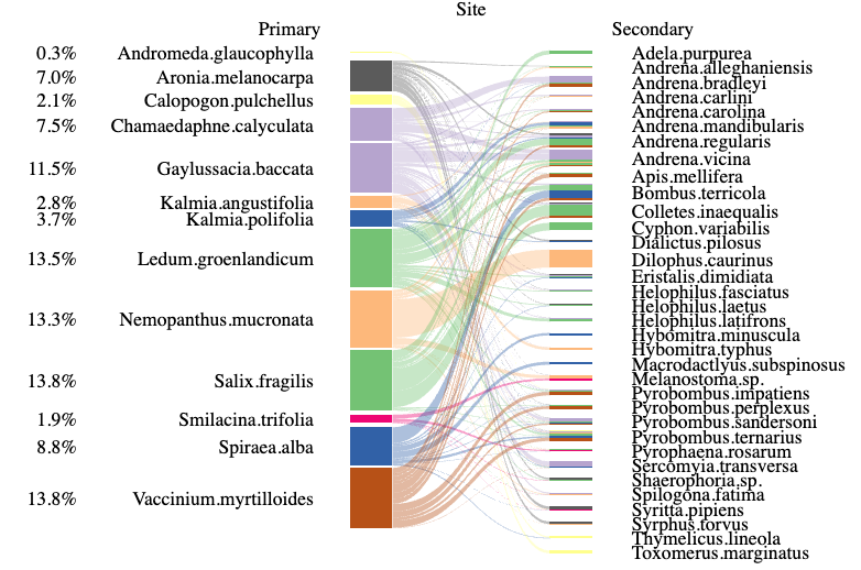
The main interest of D3 is the interactiveness, not publication-ready graphics. For this aim, it is a very nice tool and worth exploring.
8.1.2 igraph
8.1.3 ggbipart
There is the package ggbipart, on github.2222 22 See also https://pedroj.github.io/bipartite_plots/ for more code examples.
> library(devtools)> install_github(rep="pedroj/bipartite_plots")
8.1.4 multigraph
Plot several bipartite layers into one graph: see https://stackoverflow.com/questions/31366066/how-to-plot-a-bipartite-graph-in-r
8.2 Analysing the structure of bipartite networks
There are a range of packages that aim at identifying structure within networks, be it clusters/modules/compartments of a larger subset of interactions, or specific motifs of only few links. It is almost impossible to keep up with these developments, so here are just a few pointers to such packages:
- bmotif
-
A “motif” is a pattern in a network, e.g. the v-shaped link of one plant to two pollinators. This packages (Simmons et al., 2019) counts how often each of 44 such motifs is encountered in a bipartite network. This frequency distribution can then be compared to those of a null model. The majority of these motifs have no obvious ecological interpretation. For example, motif 5 is an N-shape, connecting in that N-way 2 lower with 2 higher nodes. Meaning what exactly? The brief hype following the release of this package and its main publications (Monteiro and Faria, 2016; Simmons et al., 2019; Jácome‐Flores et al., 2020) has died down a bit, and the packages has been archived on CRAN in 2022 due to unresolved code issues. Its github version can be found here: https://github.com/SimmonsBI/bmotif.
- dynsbm
- infomapecology
8.3 Multi-layer networks
This somewhat cryptic term refers to networks that are defined by different types of links, for example because links change over time (dynamic links) or because they depend on other networks (Pilosof et al., 2017). The mathematical description and analysis of such multilayer networks can be rather complex (Aleta and Moreno, 2019), and in ecology typically only relatively simple types of multilayer networks are investigated; probably the most common being multi-level networks are temporally or spatially resolved networks.
While statistically and mathematically a lot of things are conceivable, few ideas actually resonate with ecologists (i.e. in application). One idea is that networks evolve and hence change dynamically. Another is that any observed bipartite network is actually embedded in many other networks, e.g. a plant-pollinator-network may continue “into the ground” as plant-mycorrhiza networks, “into the sky” as pollinator-parasite network, and “sideways” as plant-herbivore network (Pocock et al., 2012).
Currently, bipartite does not support any such analysis (apart from a pathetic function npartite and plotweb2 for plotting stacked bipartite networks).
Packages such as robber address some of the challenges of intersecting multiple bipartite networks.
Conclusions
The analysis of bipartite networks has seen a recent explosion of applications in ecology. The R-package bipartite aims at providing a user-friendly set of function to aid the visualisation and analysis of such networks. This vignette hopefully illustrated some of the challenges and solutions to such analyses. The main take-home-message it aims to convey is that there are considerable interpretational strings attached, and that the analysis of bipartite networks is not as straightforward as one might have initially hoped.
Feedback, improvements, corrections and additions are welcomed!
The Rnw source of this document is at https://github.com/biometry/bipartite/blob/master/bipartite/vignettes/Intro2bipartite.Rnw.
References
- Year-to-year variation in the topology of a plant-pollinator interaction network. Oikos 117 (12), pp. 1796–1807. Note: 10.1111/j.0030-1299.2008.16987.x External Links: ISBN 1600-0706 Cited by: item 4.
- Problems in the measurement of evenness in ecology. Oikos 37, pp. 199–204. Cited by: item 16.
- Multilayer networks in a nutshell. Annual Review of Condensed Matter Physics 10 (1), pp. 45–62. Note: arXiv: 1804.03488 External Links: Document, ISSN 1947-5454, 1947-5462 Cited by: §8.3.
- Food web models: a plea for groups. Ecology Letters 12 (7), pp. 652–62. External Links: Document Cited by: §7.
- A consistent metric for nestedness analysis in ecological systems: reconciling concept and measurement. Oikos 117, pp. 1227–1239. External Links: Document Cited by: item 8.
- A straightforward computational approach for measuring nestedness using quantitative matrices. Environmental Modelling and Software 26, pp. 173–178. External Links: Document Cited by: item 10.
- Soil aeration status in a lowland wet grassland. Hydrological Processes 18 (2), pp. 329–341. External Links: Document Cited by: §6.1.
- The architecture of complex weighted networks. Proceedings of the National Academy of Sciences of the USA 101 (11), pp. 3747–52. External Links: Document Cited by: item 2.
- The nested assembly of plant–animal mutualistic networks. Proceedings of the National Academy of Sciences of the USA 100 (16), pp. 9383–9387. External Links: Document Cited by: item 11.
- Asymmetric coevolutionary networks facilitate biodiversity maintenance. Science 312 (5772), pp. 431–433. Cited by: item 1, item 3.
- Improved community detection in weighted bipartite networks.. Royal Society open science 3 (1), pp. 140536–140536. External Links: Document Cited by: §7.
- Quantitative descriptors of food-web matrices. Ecology 83, pp. 2394–2407. Cited by: item 13, item 14, item 15.
- What do interaction network metrics tell us about specialization and biological traits?. Ecology 89 (12), pp. 3387–99. External Links: ISSN 0012-9658, Link Cited by: §6.1, §6.2, §7.
- Measuring specialization in species interaction networks. BMC Ecology 6 (1), pp. 9. External Links: Document, ISSN 1472-6785, Link Cited by: item 18, item 18.
- Specialization, constraints, and conflicting interests in mutualistic networks. Current Biology 17 (4), pp. 341–346. External Links: ISSN 0960-9822, Document, Link Cited by: item 11, item 2.
- Why network analysis is often disconnected from community ecology: a critique and an ecologist’s guide. Basic and Applied Ecology 11, pp. 185–195. Cited by: §5.5, §6.2.
- Network analysis of 2-mode data. Social Networks 19, pp. 243–269. Cited by: item 11.
- Nested species subsets, gaps, and discrepancy. Oecologia 119 (2), pp. 256–264. External Links: Document Cited by: item 9.
- Why nestedness in mutualistic networks?. Journal of Theoretical Biology 249, pp. 307–313. Cited by: item 12.
- Sna: tools for social network analysis. Note: R package version 2.2-2 External Links: Link Cited by: §4.
- Finding community structure in very large networks. Physical Review E 70 (6), pp. 066111–066111. External Links: Document Cited by: §7.
- Herbivory: the dynamics of animal plant interactions. University of California Press, San Diego, USA. Cited by: §6.2.
- Pollination networks and functional specialization: a test using lesser antillean plant-hummingbird assemblages. Oikos 117 (5), pp. 789–793. External Links: Document Cited by: item 10.
- Effect of herbivory and plant species replacement on primary production.. The American Naturalist 155 (6), pp. 735–754. External Links: Document Cited by: §6.2.
- Understanding and planning ecological restoration of plant-pollinator networks. Ecology Letters 15, pp. 319–328. External Links: Document Cited by: item 17.
- How to be a specialist? quantifying specialisation in pollination networks. Network Biology 1, pp. 1–20. Cited by: §1.3, §5.4.
- Bipartite vignette. github. Cited by: §1.3.
- Indices, graphs and null models: analyzing bipartite ecological networks. The Open Ecology Journal 2 (1), pp. 7–24. External Links: Document Cited by: §1.3, §5.2, §5.5.2, §6.1, §6.2, §6.3, §7.
- Food webs versus interaction networks: principles, pitfalls and perspectives. In Adaptive Food Webs: Stability and Transitions of Real and Model Ecosystems, J. C. Moore, P. C. de Ruiter, K. S. McCann, and V. Wolters (Eds.), pp. 1–11. External Links: ISBN 978-1-107-18211-0, Link Cited by: §1.3.
- Introducing the bipartite package: analysing ecological networks. R News 8 (2), pp. 8–11. Cited by: §1.3.
- Identifying causes of patterns in ecological networks: opportunities and limitations. Annual Reviews in Ecology, Evolution, and Systematics 48 (September), pp. 559–84. External Links: Document Cited by: §1.3, §7.
- A method for detecting modules in quantitative bipartite networks. Methods in Ecology and Evolution 5 (1), pp. 90–98. External Links: Document Cited by: §1.3, §7.
- Food-web structure and network theory: the role of connectance and size. Proceedings of the National Academy of Sciences of the USA 99 (20), pp. 12917–22. External Links: Document Cited by: item 1.
- An introduction to the bootstrap. Chapman & Hall, London. Cited by: §6.3.
- Identifying flow modules in ecological networks using Infomap. Methods in Ecology and Evolution 12, pp. 778–786. External Links: Document Cited by: item infomapecology.
- A simple measure of niche breadth. Ecology 62 (1), pp. 27–32. External Links: Document Cited by: item 17.
- The relation between the number of species and the number of individuals in a random sample of animal population. 12, 42–58.. Journal of Animal Ecology 12, pp. 42–58. Cited by: item 14, item 13.
- Community detection in graphs. Physics Reports 486 (3-5), pp. 75–174. External Links: Document, ISSN 03701573, Link Cited by: §7.
- Weighted-interaction nestedness estimator (wine): a new estimator to calculate over frequency matrices. Environmental Modelling and Software 24 (11), pp. 1342–1346. External Links: Document Cited by: item 9.
- Buzziness as usual? questioning the global pollination crisis. Trends in Ecology and Evolution 20 (7), pp. 367–73. External Links: Document Cited by: §6.2.
- Null models in ecology. Smithsonian Institution Press. Cited by: item 1, §6.1, §6.1.
- The worldwide air transportation network: anomalous centrality, community structure, and cities’ global roles.. Proceedings of the National Academy of Sciences of the United States of America 102 (22), pp. 7794–9. External Links: Document Cited by: §6.1, §7.1.
- Null model tests of clustering of species, negative co-occurrence patterns and nestedness in meta-communities. Oikos 116 (5), pp. 818–828. External Links: Document Cited by: §6.1.
- Measurement of niche overlap and some relatives. Ecology 59 (1), pp. 67–77. Note: 0012-9658 External Links: Link Cited by: item 13.
- Interaction motifs variability in a Mediterranean palm under environmental disturbances: the mutualism–antagonism continuum. Oikos 129 (3), pp. 367–379 (en). External Links: ISSN 1600-0706, Document Cited by: item bmotif.
- Reciprocal specialization in ecological networks. Ecology Letters 12 (9), pp. 961–969. External Links: Document Cited by: §6.1, §6.2.
- Invariant properties in coevolutionary networks of plant-animal interactions. Ecology Letters 6, pp. 69–81. Cited by: item 10.
- Entropy and diversity. Oikos 113 (2), pp. 363–375. Cited by: item 16.
- Spatial segregation of specialists and generalists in bird communities. Ecology Letters 9, pp. 1237–1244. Cited by: item 8.
- Do plant–pollinator interaction networks result from stochastic processes?. Ecological Modelling 220 (5), pp. 684–693. External Links: Document, ISSN 03043800 Cited by: §6.1.
- Predator–prey ratios on cocoa along a land-use gradient in indonesia. Biodiversity and Conservation 11, pp. 683–693. Cited by: §6.2.
- A neutral-niche theory of nestedness in mutualistic networks. Oikos 117 (11), pp. 1609–1618. External Links: Document Cited by: §6.1.
- Basic notions for the analysis of large two-mode networks. Social Networks 30 (1), pp. 31–48. External Links: Document Cited by: §6.1.
- Randomization, bootstrap and monte carlo methods in biology. 2nd edition, Chapman & Hall/CRC, New York. Cited by: §6.3.
- Centrality measures and the importance of generalist species in pollination networks. Ecological Complexity 7, pp. 36–47. External Links: Document Cited by: item 2.
- Core-periphery structure in mutualistic networks: an epitaph for nestedness?. bioRxiv, pp. 2020.04.02.021691. External Links: Document Cited by: item econetwork.
- The structure of a plant-pollinator food web. Ecology Letters 2, pp. 276–280. Cited by: §7.
- Tolerance of pollination networks to species extinctions. Proceedings of the Royal Society London B 271 (1557), pp. 2605–11. External Links: Document Cited by: item 11.
- Revealing the hidden structure of dynamic ecological networks. Royal Society Open Science 4 (6), pp. 170251. External Links: Document Cited by: item dynsbm.
- The interplay between population stability and food-web topology predicts the occurrence of motifs in complex food-webs. Journal of Theoretical Biology 409, pp. 165–171. External Links: ISSN 0022-5193, Document Cited by: item bmotif.
- Toward ecologically explicit null models of nestedness. Oecologia 152 (4), pp. 763–77. External Links: Document Cited by: §6.1.
- Apparent competition and insect community structure: towards a spatial perspective. Annales Zoologici Fennici 42, pp. 449–462. Cited by: §4.
- Pollination ecology of the spring wildflower community in the deciduous forests of Piedmont North Carolina. PhD thesis, Duke University. Cited by: Figure 2, §4.
- The structure of an aphid–parasitoid community. Journal of Animal Ecology 68, pp. 346–370. Cited by: item 16.
- Finding and evaluating community structure in networks. Physical Review E 69 (2), pp. 1–15. External Links: Document Cited by: §6.1, §7.
- The structure and function of complex networks. SIAM Review 45 (2), pp. 167–256. Cited by: §7.
- Diversity indices for ecological networks: a unifying framework using hill numbers. Ecology Letters 22, pp. 737–747. External Links: Document Cited by: item econetwork.
- The modularity of pollination networks. Proceedings of the National Academy of Sciences of the USA 104, pp. 19891–19896. Cited by: §7.1.
- Triadic closure in two-mode networks: redefining the global and local cluster coefficient. arXiv, pp. 1006.0887v2. Cited by: item 5.
- Algorithm as159. an efficient method of generating r x c tables with given row and column totals. Applied Statistics 30, pp. 91–97. Cited by: §6.1.
- 2 contingency tables in ecology. Journal of Theoretical Biology 34, pp. 337–352. Cited by: item 13.
- The multilayer nature of ecological networks. Nature Ecology & Evolution 1 (4), pp. 0101–0101. External Links: Document Cited by: §8.3.
- The robustness and restoration of a network of ecological networks. Science 335, pp. 973–977. External Links: Document Cited by: §8.3.
- A conceptual framework for the evolution of ecological specialisation. Ecology Letters 14, pp. 841–851. External Links: Document Cited by: item 6.
- A comparative study of ecological specialization estimators. Methods in Ecology and Evolution 3 (3), pp. 537–544. External Links: Document Cited by: item 8, §5.4.
- Resource availability affects the structure of a natural bacteria-bacteriophage community.. Biology Letters 7 (2), pp. 201–4. External Links: Document Cited by: item 6.
- ROBustness In Network (robin): an R package for comparison and validation of communities. The R Journal 13 (1), pp. 292–309. External Links: ISSN 2073-4859 Cited by: §7.
- Island-sharing by archipelago species. Oecologia 83, pp. 560–567. Cited by: item 3.
- A new algorithm to calculate the nestedness temperature of presence-absence matrices. Journal of Biogeography 33 (5), pp. 924–935. External Links: Document Cited by: item 7.
- Linkage rules for plant–pollinator networks: trait complementarity or exploitation barriers ?. PLoS Biology 5 (2), pp. e31. External Links: Document Cited by: §6.1.
- A variance test for detecting species associations, with some example applications. Ecology 65, pp. 998–1005. Cited by: item 8.
- Food webs from the small to the large. Ecology 70, pp. 1559–1589. Cited by: item 7.
- The believing brain: from ghosts and gods to politics and conspiracies – how we construct beliefs and reinforce them as truths. St. Martin’s Griffin, New York. Cited by: item 4, footnote 16.
- Bmotif: a package for motif analyses of bipartite networks. Methods in Ecology and Evolution 0 (0). External Links: ISSN 2041-210X, Document, Link Cited by: item bmotif.
- Do resources or natural enemies drive bee population dynamics in fragmented habitats?. Ecology 89 (5), pp. 1375–1387. Cited by: §6.2.
- The checkerboard score and species distributions. Oecologia 85, pp. 74–79. Cited by: item 7.
- Competitive exclusion, or species aggregation? an aid in deciding. Oecologia 91, pp. 419–424. Cited by: item 3, item 6.
- Identifying compartments in presence-absence matrices and bipartite networks: insights into modularity measures. Journal of Biogeography 40 (4), pp. 759–768. External Links: ISSN 03050270, Document, Link Cited by: §7.
- Habitat modification alters the structure of tropical host-parasitoid food webs. Nature 445 (7124), pp. 202–5. External Links: ISSN 1476-4687, Document, Link Cited by: item 15, item 5.
- Null model analyses of specialization in plant–pollinator interactions. Ecology 84 (9), pp. 2493–2501. External Links: Document Cited by: §6.1, §7.
- Community-wide patterns of specialization in plant-pollinator interactions revealed by null models. In Plant-Pollinator Interactions: From Specialization to Generalization, N. M. Waser and J. Ollerton (Eds.), pp. 200–219. Cited by: §6.1.
- Uniting pattern and process in plant-animal mutualistic networks: a review. Annals of Botany 103 (9), pp. 1445–57. External Links: Document Cited by: §6.1.
- Species abundance and asymmetric interaction strength in ecological networks. Oikos 116 (7), pp. 1120–1127. External Links: Document Cited by: item 5, §6.2.
- Changes in interaction biodiversity induced by an introduced ungulate. Ecology Letters 6 (12), pp. 1077–1083. Cited by: §6.3.
- Generalization in pollination systems, and why it matters. Ecology 77, pp. 1043–1060. Cited by: §6.2.
- Plant-pollinator interactions: from specialization to generalization. University of Chicago Press, Chicago. Cited by: §6.2.
- Collective dynamics of ’small-world’ networks. Nature 393 (6684), pp. 440–442. External Links: Document Cited by: item 4.
Index
- adjacency matrix §3
- Alatalo interaction evenness item 16
- betweenness item 11
- C score item 7
- circularity §6.2
- closeness item 12
- connectance item 1
- discrepancy item 9
- Fisher’s alpha item 13
- for-loop §6.3
- frame2webs §3.2
- functional diversity item 17
- generality item 14
- grouplevel §5.2
- nestedrank item 4
- networklevel §5.1
- node specialisation index item 10
- normal score §6.3
- null model §6.1
- nullmodel §6.3
- Paired Differences Index item 6
- plotPAC §4
- PlottingWithBipartite §4
- plotweb §4
- ploweb §4
- pollination service index item 9
- resampling analysis §6.3
- resource range item 7
- standard score §6.3
- V ratio item 8
- visweb §4
- vulnerability item 14
- web2edges §3.3
- webs2array footnote 3
- -score §6.3