FlexMix Version 2: Finite Mixtures with Concomitant Variables and Varying and Constant Parameters
Abstract
This article is a (slightly) modified version of Grün and Leisch (2008a), published in the Journal of Statistical Software.
flexmix provides infrastructure for flexible fitting of finite mixture models in R using the expectation-maximization (EM) algorithm or one of its variants. The functionality of the package was enhanced. Now concomitant variable models as well as varying and constant parameters for the component specific generalized linear regression models can be fitted. The application of the package is demonstrated on several examples, the implementation described and examples given to illustrate how new drivers for the component specific models and the concomitant variable models can be defined.
Keywords: R, finite mixture models, generalized linear models, concomitant variables
1 Introduction
Finite mixture models are a popular technique for modelling unobserved heterogeneity or to approximate general distribution functions in a semi-parametric way. They are used in a lot of different areas such as astronomy, biology, economics, marketing or medicine. An overview on mixture models is given in Everitt and Hand (1981), Titterington et al. (1985), McLachlan and Basford (1988), Böhning (1999), McLachlan and Peel (2000) and Frühwirth-Schnatter (2006).
Version 1 of R package flexmix was introduced in Leisch (2004b). The main design principles of the package are extensibility and fast prototyping for new types of mixture models. It uses S4 classes and methods (Chambers, 1998) as implemented in the R package methods and exploits advanced features of R such as lexical scoping (Gentleman and Ihaka, 2000). The package implements a framework for maximum likelihood estimation with the expectation-maximization (EM) algorithm (Dempster et al., 1977). The main focus is on finite mixtures of regression models and it allows for multiple independent responses and repeated measurements. The EM algorithm can be controlled through arguments such as the maximum number of iterations or a minimum improvement in the likelihood to continue.
Newly introduced features in the current package version are concomitant variable models (Dayton and Macready, 1988) and varying and constant parameters in the component specific regressions. Varying parameters follow a finite mixture, i.e., several groups exist in the population which have different parameters. Constant parameters are fixed for the whole population. This model is similar to mixed-effects models (Pinheiro and Bates, 2000). The main difference is that in this application the distribution of the varying parameters is unknown and has to be estimated. Thus the model is actually closer to the varying-coefficients modelling framework (Hastie and Tibshirani, 1993), using convex combinations of discrete points as functional form for the varying coefficients.
The extension to constant and varying parameters allows for example to fit varying intercept models as given in Follmann and Lambert (1989) and Aitkin (1999a). These models are frequently applied to account for overdispersion in the data where the components follow either a binomial or Poisson distribution. The model was also extended to include nested varying parameters, i.e. this allows to have groups of components with the same parameters (Grün and Leisch, 2006; Grün, 2006).
In Section 2 the extended model class is presented together with the parameter estimation using the EM algorithm. In Section 3 examples are given to demonstrate how the new functionality can be used. An overview on the implementational details is given in Section 4. The new model drivers are presented and changes made to improve the flexibility of the software and to enable the implementation of the new features are discussed. Examples for writing new drivers for the component specific models and the concomitant variable models are given in Section 5. This paper gives a short overview on finite mixtures and the package in order to be self-contained. A more detailed introduction to finite mixtures and the package flexmix can be found in Leisch (2004b).
All computations and graphics in this paper have been done with flexmix version 2.3-21 and R version 4.6.2 using Sweave (Leisch, 2002). The newest release version of flexmix is always available from the Comprehensive R Archive Network at https://CRAN.R-project.org/package=flexmix. An up-to-date version of this paper is contained in the package as a vignette, giving full access to the R code behind all examples shown below. See help("vignette") or Leisch (2003) for details on handling package vignettes.
2 Model specification and estimation
A general model class of finite mixtures of regression models is considered in the following. The mixture is assumed to consist of components where each component follows a parametric distribution. Each component has a weight assigned which indicates the a-priori probability for an observation to come from this component and the mixture distribution is given by the weighted sum over the components. If the weights depend on further variables, these are referred to as concomitant variables.
In marketing choice behaviour is often modelled in dependence of marketing mix variables such as price, promotion and display. Under the assumption that groups of respondents with different price, promotion and display elasticities exist mixtures of regressions are fitted to model consumer heterogeneity and segment the market. Socio-demographic variables such as age and gender have often been shown to be related to the different market segments even though they generally do not perform well when used to a-priori segment the market. The relationships between the behavioural and the socio-demographic variables is then modelled through concomitant variable models where the group sizes (i.e. the weights of the mixture) depend on the socio-demographic variables.
The model class is given by
where denotes the vector of all parameters for the mixture density and is given by . denotes the response, the predictor and the concomitant variables. is the component specific density function. Multivariate variables are assumed to be dividable into subsets where the component densities are independent between the subsets, i.e. the component density is given by a product over densities which are defined for the subset variables and for . The component specific parameters are given by . Under the assumption that observations are available the dimensions of the variables are given by , for all and . In this notation denotes the dimension of the response, the dimension of the predictors and the dimension of the concomitant variables. For mixtures of GLMs each of the responses will in general be univariate, i.e. multivariate responses will be conditionally independent given the segment memberships.
For the component weights it holds that
| (1) |
where are the parameters of the concomitant variable model.
For the moment focus is given to finite mixtures where the component specific densities are from the same parametric family, i.e. for notational simplicity. If is from the exponential family of distributions and for each component a generalized linear model is fitted (McCullagh and Nelder, 1989, GLMs;) these models are also called GLIMMIX models (Wedel and DeSarbo, 1995). In this case the component specific parameters are given by where are the regression coefficients and is the dispersion parameter.
The component specific parameters are either restricted to be equal over all components, to vary between groups of components or to vary between all components. The varying between groups is referred to as varying parameters with one level of nesting. A disjoint partition , of the set is defined for the regression coefficients. is the number of groups of the regression coefficients at the nesting level. The regression coefficients are accordingly split into three groups:
where .
Similar a disjoint partition , , of can be defined for the dispersion parameters if nested varying parameters are present. denotes the number of groups of the dispersion parameters at the nesting level. This gives:
where . The nesting structure of the component specific parameters is also described in Grün and Leisch (2006).
Different concomitant variable models are possible to determine the component weights (Dayton and Macready, 1988). The mapping function only has to fulfill condition (1). In the following a multinomial logit model is assumed for the given by
with and .
2.1 Parameter estimation
The EM algorithm (Dempster et al., 1977) is the most common method for maximum likelihood estimation of finite mixture models where the number of components is fixed. The EM algorithm applies a missing data augmentation scheme. It is assumed that a latent variable exists for each observation which indicates the component membership, i.e. equals 1 if observation comes from component and 0 otherwise. Furthermore it holds that for all . In the EM algorithm these unobserved component memberships of the observations are treated as missing values and the data is augmented by estimates of the component membership, i.e. the estimated a-posteriori probabilities . For a sample of observations the EM algorithm is given by:
- E-step:
-
Given the current parameter estimates in the -th iteration, replace the missing data by the estimated a-posteriori probabilities
- M-step:
-
Given the estimates for the a-posteriori probabilities (which are functions of ), obtain new estimates of the parameters by maximizing
where
and
and can be maximized separately. The maximization of gives new estimates and the maximization of gives . is maximized separately for each using weighted ML estimation of GLMs and using weighted ML estimation of multinomial logit models.
Different variants of the EM algorithm exist such as the stochastic EM (Diebolt and Ip, 1996, SEM;) or the classification EM (Celeux and Govaert, 1992, CEM;). These two variants are also implemented in package flexmix. For both variants an additional step is made between the expectation and maximization steps. This step uses the estimated a-posteriori probabilities and assigns each observation to only one component, i.e. classifies it into one component. For SEM this assignment is determined in a stochastic way while it is a deterministic assignment for CEM. For the SEM algorithm the additional step is given by:
- S-step:
-
Given the a-posteriori probabilities draw
where denotes the multinomial distribution with success probabilities and number of trials .
Afterwards, the are used instead of the in the M-step. For the CEM the additional step is given by:
- C-step:
-
Given the a-posteriori probabilities define
Please note that in this step the observation is assigned to the component with the smallest index if the same maximum a-posteriori probability is observed for several components.
Both of these variants have been proposed to improve the performance of the EM algorithm, because the ordinary EM algorithm tends to converge rather slowly and only to a local optimum. The convergence behavior can be expected to be better for the CEM than ordinary EM algorithm, while SEM can escape convergence to a local optimum. However, the CEM algorithm does not give ML estimates because it maximizes the complete likelihood. For SEM good approximations of the ML estimator are obtained if the parameters where the maximum likelihood was encountered are used as estimates. Another possibility for determining parameter estimates from the SEM algorithm could be the mean after discarding a suitable number of burn-ins. An implementational advantage of both variants is that no weighted maximization is necessary in the M-step.
It has been shown that the values of the likelihood are monotonically increased during the EM algorithm. On the one hand this ensures the convergence of the EM algorithm if the likelihood is bounded, but on the other hand only the detection of a local maximum can be guaranteed. Therefore, it is recommended to repeat the EM algorithm with different initializations and choose as final solution the one with the maximum likelihood. Different initialization strategies for the EM algorithm have been proposed, as its convergence to the optimal solution depends on the initialization (Biernacki et al., 2003; Karlis and Xekalaki, 2003). Proposed strategies are for example to first make several runs of the SEM or CEM algorithm with different random initializations and then start the EM at the best solution encountered.
The component specific parameter estimates can be determined separately for each . For simplicity of presentation the following description assumes . If all parameter estimates vary between the component distributions they can be determined separately for each component in the M-step. However, if also constant or nested varying parameters are specified, the component specific estimation problems are not independent from each other any more. Parameters have to be estimated which occur in several or all components and hence, the parameters of the different components have to be determined simultaneously for all components. The estimation problem for all component specific parameters is then obtained by replicating the vector of observations times and defining the covariate matrix by
where is a vector of 1s of length , is the incidence matrix for each component and each nesting group and hence is of dimension , and is the identity matrix of dimension . denotes the Kronecker product and the Khatri-Rao product (i.e., the column-wise Kronecker product). are the covariates of the corresponding coefficients for . Please note that the weights used for the estimation are the a-posteriori probabilities which are stacked for all components, i.e. a vector of length is obtained.
Due to the replication of data in the case of constant or nested varying parameters the amount of memory needed for fitting the mixture model to large datasets is substantially increased and it might be easier to fit only varying coefficients to these datasets. To overcome this problem it could be considered to implement special data structures in order to avoid storing the same data multiple times for large datasets.
Before each M-step the average component sizes (over the given data points) are checked and components which are smaller than a given (relative) minimum size are omitted in order to avoid too small components where fitting problems might arise. This strategy has already been recommended for the SEM algorithm (Celeux and Diebolt, 1988) because it allows to determine the suitable number of components in an automatic way given that the a-priori specified number of components is large enough. This recommendation is based on the assumption that the redundent components will be omitted during the estimation process if the algorithm is started with too many components. If omission of small components is not desired the minimum size required can be set to zero. All components will be then retained throughout the EM algorithm and a mixture with the number of components specified in the initialization will be returned. The algorithm is stopped if the relative change in the log-likelihood is smaller than a pre-specified or the maximum number of iterations is reached.
For model selection different information criteria are available: AIC, BIC and ICL (Biernacki et al., 2000, Integrated Complete Likelihood;). They are of the form twice the negative loglikelihood plus number of parameters times where for the AIC and equals the logarithm of the number of observations for the BIC. The ICL is the same as the BIC except that the complete likelihood (where the missing class memberships are replaced by the assignments induced by the maximum a-posteriori probabilities) instead of the likelihood is used.
3 Using the new functionality
In the following model fitting and model selection in R is illustrated on several examples including mixtures of Gaussian, binomial and Poisson regression models, see also Grün (2006) and Grün and Leisch (2007).
More examples for mixtures of GLMs are provided as part of the software package through a collection of artificial and real world datasets, most of which have been previously used in the literature (see references in the online help pages). Each dataset can be loaded to R with data("name") and the fitting of the proposed models can be replayed using example("name"). Further details on these examples are given in a user guide which can be accessed using vignette("regression-examples", package="flexmix") from within R.
3.1 Artificial example
In the following the artificial dataset NPreg is used which has already been used in Leisch (2004b) to illustrate the application of package flexmix. The data comes from two latent classes of size 100 each and for each of the classes the data is drawn with respect to the following structure:
| Class 1: | |
|---|---|
| Class 2: |
with , see the left panel of Figure 1. The dataset NPreg also includes a response which is given by a generalized linear model following a Poisson distribution and using the logarithm as link function. The parameters of the mean are given for the two classes by:
| Class 1: | |
|---|---|
| Class 2: | . |
This signifies that given the response in group follows a Poisson distribution with mean , see the right panel of Figure 1.
This model can be fitted in R using the commands:
R> suppressWarnings(RNGversion("3.5.0"))R> set.seed(1802)R> library("flexmix")R> data("NPreg", package = "flexmix")R> Model_n <- FLXMRglm(yn ~ . + I(x^2))R> Model_p <- FLXMRglm(yp ~ ., family = "poisson")R> m1 <- flexmix(. ~ x, data = NPreg, k = 2, model = list(Model_n, Model_p),+ control = list(verbose = 10))
Classification: weighted 10 Log-likelihood : -1044.7688 11 Log-likelihood : -1044.7678converged
If the dimensions are independent the component specific model for multivariate observations can be specified as a list of models for each dimension.
The estimation can be controlled with the control argument which is specified with an object of class "FLXcontrol". For convenience also a named list can be provided which is used to construct and set the respective slots of the "FLXcontrol" object. Elements of the control object are classify to select ordinary EM, CEM or SEM, minprior for the minimum relative size of components, iter.max for the maximum number of iterations and verbose for monitoring. If verbose is a positive integer the log-likelihood is reported every verbose iterations and at convergence together with the number of iterations made. The default is to not report any log-likelihood information during the fitting process.
The estimated model m1 is of class "flexmix" and the result of the default plot method for this class is given in Figure 2. This plot method uses package lattice (Sarkar, 2008) and the usual parameters can be specified to alter the plot, e.g. the argument layout determines the arrangement of the panels. The returned object is of class "trellis" and the plotting can also be influenced by the arguments of its show method.
The default plot prints rootograms (i.e., a histogram of the square root of counts) of the a-posteriori probabilities of each observation separately for each component. For each component the observations with a-posteriori probabilities less than a pre-specified (default is ) for this component are omitted in order to avoid that the bar at zero dominates the plot (Leisch, 2004a). Please note that the labels of the y-axis report the number of observations in each bar, i.e. the squared values used for the rootograms.
More detailed information on the estimated parameters with respect to standard deviations and significance tests can be obtained with function refit(). This function determines the variance-covariance matrix of the estimated parameters by using the inverted negative Hesse matrix as computed by the general purpose optimizer optim() on the full likelihood of the model. optim() is initialized in the solution obtained with the EM algorithm. For mixtures of GLMs we also implemented the gradient, which speeds up convergence and gives more precise estimates of the Hessian.
Naturally, function refit() will also work for models which have been determined by applying some model selection strategy depending on the data (AIC, BIC, …). The same caution is necessary as when using summary() on standard linear models selected using step(): The p-values shown are not correct because they have not been adjusted for the fact that the same data are used to select the model and compute the p-values. So use them only in an exploratory manner in this context, see also Harrell (2001) for more details on the general problem.
The returned object can be inspected using summary() with arguments which to specify if information for the component model or the concomitant variable model should be shown and model to indicate for which dimension of the component models this should be done. Selecting model=1 gives the parameter estimates for the dimension where the response variable follows a Gaussian distribution.
R> m1.refit <- refit(m1)R> summary(m1.refit, which = "model", model = 1)
$Comp.1 Estimate Std. Error z value Pr(>|z|)(Intercept) 14.58965 1.24635 11.706 < 2.2e-16 ***x 9.91572 0.55294 17.933 < 2.2e-16 ***I(x^2) -0.97578 0.05201 -18.762 < 2.2e-16 ***---Signif. codes:0 '***' 0.001 '**' 0.01 '*' 0.05 '.' 0.1 ' ' 1$Comp.2 Estimate Std. Error z value Pr(>|z|)(Intercept) -0.140549 0.961868 -0.1461 0.8838x 4.732610 0.474428 9.9754 <2e-16 ***I(x^2) 0.042722 0.046890 0.9111 0.3622---Signif. codes:0 '***' 0.001 '**' 0.01 '*' 0.05 '.' 0.1 ' ' 1
The default plot method for the refitted "flexmix" object depicts the estimated coefficients with corresponding confidence intervals and is given in Figure 3. It can be seen that for the first model the confidence intervals of the coefficients of the intercept and the quadratic term of x overlap with zero.
A model where these coefficients are set to zero can be estimated with the model driver function FLXMRglmfix() and the following commands for specifying the nesting structure. The argument nested needs input for the number of components in each group (given by k) and the formula which determines the model matrix for the nesting (given by formula). This information can be provided in a named list.
For the restricted model the element k is a vector with two 1s
because each of the components has different parameters. The formulas
specifying the model matrices of these coefficients are
~ 1 + I(x^2) for an intercept and a quadratic term of
for component 1 and ~ 0 for no additional coefficients for
component 2. The EM algorithm is initialized in the previously fitted
model by passing the posterior probabilities in the argument
cluster.
R> Model_n2 <- FLXMRglmfix(yn ~ . + 0, nested = list(k = c(1, 1),+ formula = c(~ 1 + I(x^2), ~ 0)))R> m2 <- flexmix(. ~ x, data = NPreg, cluster = posterior(m1),+ model = list(Model_n2, Model_p))R> m2
Call:flexmix(formula = . ~ x, data = NPreg, cluster = posterior(m1), model = list(Model_n2, Model_p))Cluster sizes: 1 2 96 104convergence after 3 iterations
Model selection based on the BIC would suggest the smaller model which also corresponds to the true underlying model.
R> c(BIC(m1), BIC(m2))
[1] 2158.414 2149.956
3.2 Beta-blockers dataset
The dataset is analyzed in Aitkin (1999a); Aitkin (1999b) using a finite mixture of binomial regression models. Furthermore, it is described in McLachlan and Peel (2000, p. 165). The dataset is from a 22-center clinical trial of beta-blockers for reducing mortality after myocardial infarction. A two-level model is assumed to represent the data, where centers are at the upper level and patients at the lower level. The data is illustrated in Figure 4.
First, the center information is ignored and a binomial logit regression model with treatment as covariate is fitted using glm, i.e. and it is assumed that the different centers are comparable:
R> data("betablocker", package = "flexmix")R> betaGlm <- glm(cbind(Deaths, Total - Deaths) ~ Treatment,+ family = "binomial", data = betablocker)R> betaGlm
Call: glm(formula = cbind(Deaths, Total - Deaths) ~ Treatment, family = "binomial", data = betablocker)Coefficients: (Intercept) TreatmentTreated -2.1971 -0.2574Degrees of Freedom: 43 Total (i.e. Null); 42 ResidualNull Deviance: 333Residual Deviance: 305.8 AIC: 527.2
The residual deviance suggests that overdispersion is present in the data. In the next step the intercept is allowed to follow a mixture distribution given the centers. This signifies that the component membership is fixed for each center. This grouping is specified in R by adding | Center to the formula similar to the notation used in nlme (Pinheiro and Bates, 2000). Under the assumption of homogeneity within centers identifiability of the model class can be ensured as induced by the sufficient conditions for identifability given in Follmann and Lambert (1991) for binomial logit models with varying intercepts and Grün and Leisch (2008b) for multinomial logit models with varying and constant parameters. In order to determine the suitable number of components, the mixture is fitted with different numbers of components.
R> betaMixFix <- stepFlexmix(cbind(Deaths, Total - Deaths) ~ 1 | Center,+ model = FLXMRglmfix(family = "binomial", fixed = ~ Treatment),+ k = 2:4, nrep = 5, data = betablocker)
2 : * * * * *3 : * * * * *4 : * * * * *
The returned object is of class "stepFlexmix" and printing the object gives the information on the number of iterations until termination of the EM algorithm, a logical indicating if the EM algorithm has converged, the log-likelihood and some model information criteria. The plot method compares the fitted models using the different model information criteria.
R> betaMixFix
Call:stepFlexmix(cbind(Deaths, Total - Deaths) ~ 1 | Center, model = FLXMRglmfix(family = "binomial", fixed = ~Treatment), data = betablocker, k = 2:4, nrep = 5) iter converged k k0 logLik AIC BIC ICL2 12 TRUE 2 2 -181.3308 370.6617 377.7984 380.21053 9 TRUE 3 3 -159.3605 330.7210 341.4262 343.32574 13 TRUE 4 4 -158.2465 332.4929 346.7664 354.4909
A specific "flexmix" model contained in the "stepFlexmix" object can be selected using getModel() with argument which to specify the selection criterion. The best model with respect to the BIC is selected with:
R> betaMixFix_3 <- getModel(betaMixFix, which = "BIC")R> betaMixFix_3 <- relabel(betaMixFix_3, "model", "Intercept")
The components of the selected model are ordered with respect to the estimated intercept values.
In this case a model with three components is selected with respect to the BIC. The fitted values for the model with three components are given in Figure 4 separately for each component and the treatment and control groups.
The fitted parameters of the component specific models can be accessed with:
R> parameters(betaMixFix_3)
Comp.1 Comp.2 Comp.3coef.TreatmentTreated -0.2581849 -0.2581849 -0.2581849coef.(Intercept) -2.8336816 -2.2501814 -1.6097872
Please note that the coefficients of variable Treatment are the same for all three components.
The variable Treatment can also be included in the varying part of the model. This signifies that a mixture distribution is assumed where for each component different values are allowed for the intercept and the treatment coefficient. This mixture distribution can be specified using function FLXMRglm(). Again it is assumed that the heterogeneity is only between centers and therefore the aggregated data for each center can be used.
R> betaMix <- stepFlexmix(cbind(Deaths, Total - Deaths) ~ Treatment | Center,+ model = FLXMRglm(family = "binomial"), k = 3, nrep = 5,+ data = betablocker)
3 : * * * * *
R> betaMix <- relabel(betaMix, "model", "Treatment")R> parameters(betaMix)
Comp.1 Comp.2 Comp.3coef.(Intercept) -1.5800031 -2.2476980 -2.91633722coef.TreatmentTreated -0.3248497 -0.2630017 -0.08047829
R> c(BIC(betaMixFix_3), BIC(betaMix))
[1] 341.4262 346.8925
The difference between model betaMix and betaMixFix_3 is that the treatment coefficients are the same for all three components for betaMixFix_3 while they have different values for betaMix which can easily be seen when comparing the fitted component specific parameters. The larger model betaMix which also allows varying parameters for treatment has a higher BIC and therefore the smaller model betaMixFix_3 would be preferred.
The default plot for "flexmix" objects gives a rootogram of the posterior probabilities for each component. Argument mark can be used to inspect with which components the specified component overlaps as all observations are coloured in the different panels which are assigned to this component based on the maximum a-posteriori probabilities.
The rootogram indicates that the components are well separated. In Figure 5 it can be seen that component 1 is completely separated from the other two components, while Figure 6 shows that component 2 has a slight overlap with both other components.
The cluster assignments using the maximum a-posteriori probabilities are obtained with:
R> table(clusters(betaMix))
1 2 310 24 10
The estimated probabilities of death for each component for the treated patients and those in the control group can be obtained with:
R> predict(betaMix,+ newdata = data.frame(Treatment = c("Control", "Treated")))
$Comp.1 [,1]1 0.17079502 0.1295602$Comp.2 [,1]1 0.095548222 0.07511149$Comp.3 [,1]1 0.051351842 0.04756995
or by obtaining the fitted values for two observations (e.g. rows 1 and 23) with the desired levels of the predictor Treatment
R> betablocker[c(1, 23), ]
Deaths Total Center Treatment1 3 39 1 Control23 3 38 1 Treated
R> fitted(betaMix)[c(1, 23), ]
Comp.1 Comp.2 Comp.3[1,] 0.1707950 0.09554822 0.05135184[2,] 0.1295602 0.07511149 0.04756995
A further analysis of the model is possible with function refit() which returns the estimated coefficients together with the standard deviations, z-values and corresponding p-values. Please note that the p-values are only approximate in the sense that they have not been corrected for the fact that the data has already been used to determine the specific fitted model.
R> summary(refit(betaMix))
$Comp.1 Estimate Std. Error z value Pr(>|z|)(Intercept) -1.579965 0.065997 -23.9401 < 2.2e-16TreatmentTreated -0.324833 0.092882 -3.4973 0.0004701(Intercept) ***TreatmentTreated ***---Signif. codes:0 '***' 0.001 '**' 0.01 '*' 0.05 '.' 0.1 ' ' 1$Comp.2 Estimate Std. Error z value Pr(>|z|)(Intercept) -2.247678 0.045181 -49.7481 < 2.2e-16TreatmentTreated -0.262990 0.065598 -4.0091 6.095e-05(Intercept) ***TreatmentTreated ***---Signif. codes:0 '***' 0.001 '**' 0.01 '*' 0.05 '.' 0.1 ' ' 1$Comp.3 Estimate Std. Error z value Pr(>|z|)(Intercept) -2.91634 0.09921 -29.3958 <2e-16 ***TreatmentTreated -0.08048 0.14104 -0.5706 0.5683---Signif. codes:0 '***' 0.001 '**' 0.01 '*' 0.05 '.' 0.1 ' ' 1
Given the estimated treatment coefficients we now also compare this model to a model where the treatment coefficient is assumed to be the same for components 1 and 2. Such a model is specified using the model driver FLXMRglmfix(). As the first two components are assumed to have the same coeffcients for treatment and for the third component the coefficient for treatment shall be set to zero the argument nested has k = c(2,1) and formula = c(˜Treatment, ˜).
R> ModelNested <- FLXMRglmfix(family = "binomial", nested = list(k = c(2, 1),+ formula = c(~ Treatment, ~ 0)))R> betaMixNested <- flexmix(cbind(Deaths, Total - Deaths) ~ 1 | Center,+ model = ModelNested, k = 3, data = betablocker,+ cluster = posterior(betaMix))R> parameters(betaMixNested)
$Comp.1coef.TreatmentTreated coef.(Intercept) -0.2837779 -1.5985089$Comp.2coef.TreatmentTreated coef.(Intercept) -0.2837779 -2.2379835$Comp.3coef.(Intercept) -2.956159
R> c(BIC(betaMix), BIC(betaMixNested), BIC(betaMixFix_3))
[1] 346.8925 339.9429 341.4262
The comparison of the BIC values suggests that the nested model with the same treatment effect for two components and no treatment effect for the third component is the best.
3.3 Productivity of Ph.D. students in biochemistry
This dataset is taken from Long (1990). It contains 915 observations from academics who obtained their Ph.D. degree in biochemistry in the 1950s and 60s. It includes 421 women and 494 men. The productivity was measured by counting the number of publications in scientific journals during the three years period ending the year after the Ph.D. was received. In addition data on the productivity and the prestige of the mentor and the Ph.D. department was collected. Two measures of family characteristics were recorded: marriage status and number of children of age 5 and lower by the year of the Ph.D.
First, mixtures with one, two and three components and only varying parameters are fitted, and the model minimizing the BIC is selected. This is based on the assumption that unobserved heterogeneity is present in the data due to latent differences between the students in order to be productive and achieve publications. Starting with the most general model to determine the number of components using information criteria and checking for possible model restrictions after having the number of components fixed is a common strategy in finite mixture modelling (Wang et al., 1996, see). Function refit() is used to determine confidence intervals for the parameters in order to choose suitable alternative models. However, it has to be noted that in the course of the procedure these confidence intervals will not be correct any more because the specific fitted models have already been determined using the same data.
R> data("bioChemists", package = "flexmix")R> Model1 <- FLXMRglm(family = "poisson")R> ff_1 <- stepFlexmix(art ~ ., data = bioChemists, k = 1:3, model = Model1)
1 : * * *2 : * * *3 : * * *
R> ff_1 <- getModel(ff_1, "BIC")
The selected model has 2 components. The estimated coefficients of the components are given in Figure 7 together with the corresponding 95% confidence intervals using the plot method for objects returned by refit(). The plot shows that the confidence intervals of the parameters for kid5, mar, ment and phd overlap for the two components. In a next step a mixture with two components is therefore fitted where only a varying intercept and a varying coefficient for fem is specified and all other coefficients are constant. The EM algorithm is initialized with the fitted mixture model using posterior().
R> Model2 <- FLXMRglmfix(family = "poisson", fixed = ~ kid5 + mar + ment)R> ff_2 <- flexmix(art ~ fem + phd, data = bioChemists,+ cluster = posterior(ff_1), model = Model2)R> c(BIC(ff_1), BIC(ff_2))
[1] 3212.991 3200.071
If the BIC is used for model comparison the smaller model including only varying coefficients for the intercept and fem is preferred. The coefficients of the fitted model can be obtained using refit():
R> summary(refit(ff_2))
$Comp.1 Estimate Std. Error z value Pr(>|z|)kid5 -0.2070933 0.0521307 -3.9726 7.11e-05 ***marMarried 0.1646178 0.0768505 2.1421 0.0321892 *ment 0.0274302 0.0032899 8.3377 < 2.2e-16 ***(Intercept) -0.4782683 0.2203178 -2.1708 0.0299455 *femWomen 0.6045078 0.1822082 3.3177 0.0009077 ***phd 0.0775564 0.0408161 1.9001 0.0574148 .---Signif. codes:0 '***' 0.001 '**' 0.01 '*' 0.05 '.' 0.1 ' ' 1$Comp.2 Estimate Std. Error z value Pr(>|z|)kid5 -0.2070933 0.0521307 -3.9726 7.110e-05 ***marMarried 0.1646178 0.0768505 2.1421 0.03219 *ment 0.0274302 0.0032899 8.3377 < 2.2e-16 ***(Intercept) 1.3208461 0.2337508 5.6507 1.598e-08 ***femWomen -2.2054873 0.4313329 -5.1132 3.168e-07 ***phd -0.0818211 0.0554627 -1.4752 0.14015---Signif. codes:0 '***' 0.001 '**' 0.01 '*' 0.05 '.' 0.1 ' ' 1
It can be seen that the coefficient of phd does for both components not differ significantly from zero and might be omitted. This again improves the BIC.
R> Model3 <- FLXMRglmfix(family = "poisson", fixed = ~ kid5 + mar + ment)R> ff_3 <- flexmix(art ~ fem, data = bioChemists, cluster = posterior(ff_2),+ model = Model3)R> c(BIC(ff_2), BIC(ff_3))
[1] 3200.071 3192.816
The coefficients of the restricted model without phd are given in Figure 8.
An alternative model would be to assume that gender does not directly influence the number of articles but has an impact on the segment sizes.
R> Model4 <- FLXMRglmfix(family = "poisson", fixed = ~ kid5 + mar + ment)R> ff_4 <- flexmix(art ~ 1, data = bioChemists, cluster = posterior(ff_2),+ concomitant = FLXPmultinom(~ fem), model = Model4)R> parameters(ff_4)
Comp.1 Comp.2coef.kid5 -0.1819162 -0.1819162coef.marMarried 0.1883990 0.1883990coef.ment 0.0288501 0.0288501coef.(Intercept) -0.2583828 0.9950050
R> summary(refit(ff_4), which = "concomitant")
$Comp.2 Estimate Std. Error z value Pr(>|z|)(Intercept) -1.02262 0.28385 -3.6027 0.0003149 ***femWomen -0.61281 0.27280 -2.2464 0.0246782 *---Signif. codes:0 '***' 0.001 '**' 0.01 '*' 0.05 '.' 0.1 ' ' 1
R> BIC(ff_4)
[1] 3182.328This suggests that the proportion of women is lower in the second component which is the more productive segment.
The alternative modelling strategy where homogeneity is assumed at the beginning and a varying interept is added if overdispersion is observed leads to the following model which is the best with respect to the BIC.
R> Model5 <- FLXMRglmfix(family = "poisson", fixed = ~ kid5 + ment + fem)R> ff_5 <- flexmix(art ~ 1, data = bioChemists, cluster = posterior(ff_2),+ model = Model5)R> BIC(ff_5)
[1] 3174.266
In Figure 9 the estimated distribution of productivity for model ff_5 are given separately for men and women as well as for each component where for all other variables the mean values are used for the numeric variables and the most frequent category for the categorical variables. The two components differ in that component 1 contains the students who publish no article or only a single article, while the students in component 2 write on average several articles. With a constant coefficient for gender women publish less articles than men in both components.
This example shows that different optimal models are chosen for different modelling procedures. However, the distributions induced by the different variants of the model class may be similar and therefore it is not suprising that they then will have similar BIC values.
4 Implementation
The new features extend the available model class described in Leisch (2004b) by providing infrastructure for concomitant variable models and for fitting mixtures of GLMs with varying and constant parameters for the component specific parameters. The implementation of the extensions of the model class made it necessary to define a better class structure for the component specific models and to modify the fit functions flexmix() and FLXfit().
An overview on the S4 class structure of the package is given in Figure 10. There is a class for unfitted finite mixture distributions given by "FLXdist" which contains a list of "FLXM" objects which determine the component specific models, a list of "FLXcomponent" objects which specify functions to determine the component specific log-likelihoods and predictions and which contain the component specific parameters, and an object of class "FLXP" which specifies the concomitant variable model. Class "flexmix" extends "FLXdist". It represents a fitted finite mixture distribution and it contains the information about the fitting with the EM algorithm in the object of class "FLXcontrol". Repeated fitting with the EM algorithm with different number of components is provided by function stepFlexmix() which returns an object of class "stepFlexmix". Objects of class "stepFlexmix" contain the list of the fitted mixture models for each number of components in the slot "models".
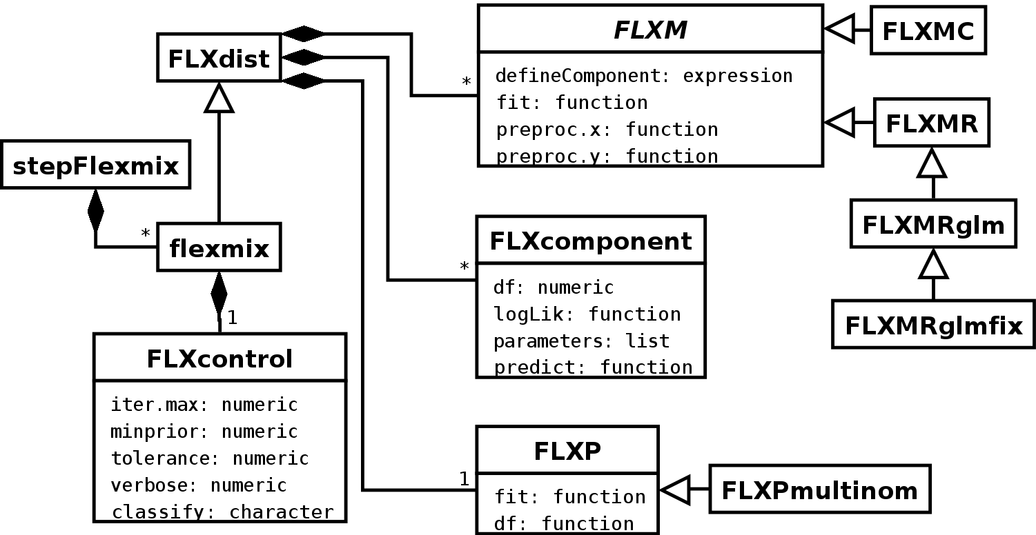
For the component specific model a virtual class "FLXM" is introduced which (currently) has two subclasses: "FLXMC" for model-based clustering and "FLXMR" for clusterwise regression, where predictor variables are given. Additional slots have been introduced to allow for data preprocessing and the construction of the components was separated from the fit and is implemented using lexical scoping (Gentleman and Ihaka, 2000) in the slot defineComponent. "FLXMC" has an additional slot dist to specify the name of the distribution of the variable. In the future functionality shall be provided for sampling from a fitted or unfitted finite mixture. Using this slot observations can be generated by using the function which results from adding an r at the beginnning of the distribution name. This allows to only implement the (missing) random number generator functions and otherwise use the same method for sampling from mixtures with component specific models of class "FLXMC".
For flexmix() and FLXfit() code blocks which are model dependent have been identified and different methods implemented. Finite mixtures of regressions with varying, nested and constant parameters were a suitable model class for this identification task as they are different from models previously implemented. The main differences are:
- •
The number of components is related to the component specific model and the omission of small components during the EM algorithm impacts on the model.
- •
The parameters of the component specific models can not be determined separately in the M-step and a joint model matrix is needed.
This makes it also necessary to have different model dependent methods for fitted() which extracts the fitted values from a "flexmix" object, predict() which predicts new values for a "flexmix" object and refit() which refits an estimated model to obtain additional information for a "flexmix" object.
4.1 Component specific models with varying and constant parameters
A new M-step driver is provided which fits finite mixtures of GLMs with constant and nested varying parameters for the coefficients and the dispersion parameters. The class "FLXMRglmfix" returned by the driver FLXMRglmfix() has the following additional slots with respect to "FLXMRglm":
- design:
-
An incidence matrix indicating which columns of the model matrix are used for which component, i.e. .
- nestedformula:
-
An object of class "FLXnested" containing the formula for the nested regression coefficients and the number of components in each , .
- fixed:
-
The formula for the constant regression coefficients.
- variance:
-
A logical indicating if different variances shall be estimated for the components following a Gaussian distribution or a vector specifying the nested structure for estimating these variances.
The difference between estimating finite mixtures including only varying parameters using models specified with FLXMRglm() and those with varying and constant parameters using function FLXMRglmfix() is hidden from the user, as only the specified model is different. The fitted model is also of class "flexmix" and can be analyzed using the same functions as for any model fitted using package flexmix. The methods used are the same except if the slot containing the model is accessed and method dispatching is made via the model class. New methods are provided for models of class "FLXMRglmfix" for functions refit(), fitted() and predict() which can be used for analyzing the fitted model.
The implementation allows repeated measurements by specifying a grouping variable in the formula argument of flexmix(). Furthermore, it has to be noticed that the model matrix is determined by updating the formula of the varying parameters successively with the formula of the constant and then of the nested varying parameters. This ensures that if a mixture distribution is fitted for the intercept, the model matrix of a categorical variable includes only the remaining columns for the constant parameters to have full column rank. However, this updating scheme makes it impossible to estimate a constant intercept while allowing varying parameters for a categorical variable.
For this model one big model matrix is constructed where the observations are repeated times and suitable columns of zero added. The coefficients of all components are determined simultaneously in the M-step, while if only varying parameters are specified the maximization of the likelihood is made separately for all components. For large datasets the estimation of a combination of constant and varying parameters might therefore be more challenging than only varying parameters.
4.2 Concomitant variable models
For representing concomitant variable models the class "FLXP" is defined. It specifies how the concomitant variable model is fitted using the concomitant variable model matrix as predictor variables and the current a-posteriori probability estimates as response variables. The object has the following slots:
- fit:
-
A function (x, y, ...) returning the fitted values for the component weights during the EM algorithm.
- refit:
-
A function (x, y, ...) used for refitting the model.
- df:
-
A function (x, k, ...) returning the degrees of freedom used for estimating the concomitant variable model given the model matrix x and the number of components k.
- x:
-
A matrix containing the model matrix of the concomitant variables.
- formula:
-
The formula for determining the model matrix x.
- name:
-
A character string describing the model, which is only used for print output.
Two constructor functions for concomitant variable models are provided at the moment. FLXPconstant() is for constant component weights without concomitant variables and for multinomial logit models FLXPmultinom() can be used. FLXPmultinom() has its own class "FLXPmultinom" which extends "FLXP" and has an additional slot coef for the fitted coefficients. The multinomial logit models are fitted using package nnet (Venables and Ripley, 2002).
4.3 Further changes
The estimation of the model with the EM algorithm was improved by adapting the variants to correspond to the CEM and SEM variants as outlined in the literature. To make this more explicit it is now also possible to use "CEM" or "SEM" to specify an EM variant in the classify argument of the "FLXcontrol" object. Even though the SEM algorithm can in general not be expected to converge the fitting procedure is also terminated for the SEM algorithm if the change in the relative log-likelhood is smaller than the pre-specified threshold. This is motivated by the fact that for well separated clusters the posteriors might converge to an indicator function with all weight concentrated in one component. The fitted model with the maximum likelihood encountered during the SEM algorithm is returned.
For discrete data in general multiple observations with the same values are given in a dataset. A weights argument was added to the fitting function flexmix() in order to avoid repeating these observations in the provided dataset. The specification is through a formula in order to allow selecting a column of the data frame given in the data argument. The weights argument allows to avoid replicating the same observations and hence enables more efficient memory use in these applications. This possibitliy is especially useful in the context of model-based clustering for mixtures of Poisson distributions or latent class analysis with multivariate binary observations.
In order to be able to apply different initialization strategies such as for example first running several different random initializations with CEM and then switching to ordinary EM using the best solution found by CEM for initialization a posterior() function was implemented. posterior() also takes a newdata argument and hence, it is possible to apply subset strategies for large datasets as suggested in Wehrens et al. (2004). The returned matrix of the posterior probabilities can be used to specify the cluster argument for flexmix() and the posteriors are then used as weights in the first M-step.
The default plot methods now use trellis graphics as implemented in package lattice (Sarkar, 2008). Users familiar with the syntax of these graphics and with the plotting and printing arguments will find the application intuitive as a lot of plotting arguments are passed to functions from lattice as for example xyplot() and histogram(). In fact only new panel, pre-panel and group-panel functions were implemented. The returned object is of class "trellis" and the show method for this class is used to create the plot.
Function refit() was modified and has now two different estimation methods: "optim" and "mstep". The default method "optim" determines the variance-covariance matrix of the parameters from the inverse Hessian of the full log-likelihood. The general purpose optimizer optim() is used to maximize the log-likelihood and initialized in the solution obtained with the EM algorithm. For mixtures of GLMs there are also functions implemented to determine the gradient which can be used to speed up convergence.
The second method "mstep" is only a raw approximation. It performs an M-step where the a-posteriori probabilities are treated as given instead of estimated and returns for the component specific models nearly complete "glm" objects which can be further analyzed. The advantage of this method is that the return value is basically a list of standard "glm" objects, such that the regular methods for this class can be used.
5 Writing your own drivers
Two examples are given in the following to demonstrate how new drivers can be provided for concomitant variable models and for component specific models. Easy extensibility is one of the main implementation aims of the package and it can be seen that writing new drivers requires only a few lines of code for providing the constructor functions which include the fit functions.
5.1 Component specific models: Zero-inflated models
In Poisson or binomial regression models it can be often encountered that the observed number of zeros is higher than expected. A mixture with two components where one has mean zero can be used to model such data. These models are also referred to as zero-inflated models (Böhning et al., 1999, see for example). A generalization of this model class would be to fit mixtures with more than two components where one component has a mean fixed at zero. So this model class is a special case of a mixture of generalized linear models where (a) the family is restricted to Poisson and binomial and (b) the parameters of one component are fixed. For simplicity the implementation assumes that the component with mean zero is the first component. In addition we assume that the model matrix contains an intercept and to have the first component absorbing the access zeros the coefficient of the intercept is set to and all other coefficients are set to zero.
Hence, to implement this model using package flexmix an appropriate model class is needed with a corresponding convenience function for construction. During the fitting of the EM algorithm using flexmix() different methods for this model class are needed when determining the model matrix (to check the presence of an intercept), to check the model after a component is removed and for the M-step to account for the fact that the coefficients of the first component are fixed. For all other methods those available for "FLXMRglm" can be re-used. The code is given in Figure 11.
The model class "FLXMRziglm" is defined as extending "FLXMRglm" in order to be able to inherit methods from this model class. For construction of a "FLXMRziglm" class the convenicence function FLXMRziglm() is used which calls FLXMRglm(). The only differences are that the family is restricted to binomial or Poisson, that a different name is assigned and that an object of the correct class is returned.
The presence of the intercept in the model matrix is checked in FLXgetModelmatrix() after using the method available for "FLXMRglm" models as indicated by the call to callNextMethod(). During the EM algorithm FLXremoveComponent() is called if one component is removed. For this model class it checks if the first component has been removed and if this is the case the model class is changed to "FLXMRglm".
In the M-step the coefficients of the first component are fixed and not estimated, while for the remaining components the M-step of "FLXMRglm" objects can be used. During the EM algorithm FLXmstep() is called to perform the M-step and returns a list of "FLXcomponent" objects with the fitted parameters. A new method for this function is needed for "FLXMRziglm" objects in order to account for the fixed coefficients in the first component, i.e. for the first component the "FLXcomponent" object is constructed and concatenated with the list of "FLXcomponent" objects returned by using the FLXmstep() method for "FLXMRglm" models for the remaining components.
Similar modifications are necessary in order to be able to use refit() for this model class. The code for implementing the refit() method using optim() for "FLXMRziglm" is not shown, but can be inspected in the source code of the package.
5.1.1 Example: Using the driver
This new M-step driver can be used to estimate a zero-inflated Poisson model to the data given in Böhning et al. (1999). The dataset dmft consists of count data from a dental epidemiological study for evaluation of various programs for reducing caries collected among school children from an urban area of Belo Horizonte (Brazil). The variables included are the number of decayed, missing or filled teeth (DMFT index) at the beginning and at the end of the observation period, the gender, the ethnic background and the specific treatment for 797 children.
The model can be fitted with the new driver function using the following commands:
R> data("dmft", package = "flexmix")R> Model <- FLXMRziglm(family = "poisson")R> Fitted <- flexmix(End ~ log(Begin + 0.5) + Gender + Ethnic + Treatment,+ model = Model, k = 2 , data = dmft, control = list(minprior = 0.01))R> summary(refit(Fitted))
$Comp.2 Estimate Std. Error z value Pr(>|z|)(Intercept) -0.1470652 0.0963031 -1.5271 0.126734log(Begin + 0.5) 0.7303431 0.0402403 18.1496 < 2.2e-16Gendermale 0.0068805 0.0550486 0.1250 0.900531Ethnicwhite 0.0500281 0.0592975 0.8437 0.398848Ethnicblack -0.0472578 0.0899984 -0.5251 0.599516Treatmenteduc -0.2371848 0.0905877 -2.6183 0.008837Treatmentall -0.3277747 0.1011637 -3.2400 0.001195Treatmentenrich 0.0172642 0.0838730 0.2058 0.836918Treatmentrinse -0.2414627 0.0871032 -2.7721 0.005569Treatmenthygiene -0.1026315 0.0916676 -1.1196 0.262882(Intercept)log(Begin + 0.5) ***GendermaleEthnicwhiteEthnicblackTreatmenteduc **Treatmentall **TreatmentenrichTreatmentrinse **Treatmenthygiene---Signif. codes:0 '***' 0.001 '**' 0.01 '*' 0.05 '.' 0.1 ' ' 1
Please note that Böhning et al. (1999) added the predictor log(Begin + 0.5) to serve as an offset in order to be able to analyse the improvement in the DMFT index from the beginning to the end of the study. The linear predictor with the offset subtracted is intended to be an estimate for . This is justified by the fact that for a Poisson distributed variable with mean between 1 and 10 it holds that is approximately equal to . can therefore be seen as an estimate for .
The estimated coefficients with corresponding confidence intervals are given in Figure 12. As the coefficients of the first component are restricted a-priori to minus infinity for the intercept and to zero for the other variables, they are of no interest and only the second component is plotted. The box ratio can be modified as for barchart() in package lattice. The code to produce this plot is given by:
R> print(plot(refit(Fitted), components = 2, box.ratio = 3))
5.2 Concomitant variable models
If the concomitant variable is a categorical variable, the multinomial logit model is equivalent to a model where the component weights for each level of the concomitant variable are determined by the mean values of the a-posteriori probabilities. The driver which implements this "FLXP" model is given in Figure 13. A name for the driver has to be specified and a fit() function. In the fit() function the mean posterior probability for all observations with the same covariate points is determined, assigned to the corresponding observations and the full new a-posteriori probability matrix returned. By contrast refit() only returns the new a-posteriori probability matrix for the number of unique covariate points.
5.2.1 Example: Using the driver
If the concomitant variable model returned by myConcomitant() is used for the artificial example in Section 3 the same fitted model is returned as if a multinomial logit model is specified. An advantage is that in this case no problems occur if the fitted probabilities are close to zero or one.
R> Concomitant <- FLXPmultinom(~ yb)R> MyConcomitant <- myConcomitant(~ yb)R> set.seed(1234)R> m2 <- flexmix(. ~ x, data = NPreg, k = 2, model = list(Model_n, Model_p),+ concomitant = Concomitant)R> m3 <- flexmix(. ~ x, data = NPreg, k = 2, model = list(Model_n, Model_p),+ cluster = posterior(m2), concomitant = MyConcomitant)
R> summary(m2)
Call:flexmix(formula = . ~ x, data = NPreg, k = 2, model = list(Model_n, Model_p), concomitant = Concomitant) prior size post>0 ratioComp.1 0.5 100 181 0.552Comp.2 0.5 100 185 0.541'log Lik.' -1085.995 (df=14)AIC: 2199.99 BIC: 2246.166
R> summary(m3)
Call:flexmix(formula = . ~ x, data = NPreg, k = 2, cluster = posterior(m2), model = list(Model_n, Model_p), concomitant = MyConcomitant) prior size post>0 ratioComp.1 0.5 100 181 0.552Comp.2 0.5 100 185 0.541'log Lik.' -1085.994 (df=14)AIC: 2199.988 BIC: 2246.164
For comparing the estimated component weights for each value of the following function can be used:
R> determinePrior <- function(object) {+ object@concomitant@fit(object@concomitant@x,+ posterior(object))[!duplicated(object@concomitant@x), ]+ }
R> determinePrior(m2)
[,1] [,2]1 0.1121413 0.887858684 0.9288377 0.07116225
R> determinePrior(m3)
[,1] [,2]1 0.1123502 0.887649792 0.9288742 0.07112579Obviously the fitted values of the two models correspond to each other.
6 Summary and outlook
Package flexmix was extended to cover finite mixtures of GLMs with (nested) varying and constant parameters. This allows for example the estimation of varying intercept models. In order to be able to characterize the components given some variables concomitant variable models can be estimated for the component weights.
The implementation of these extensions have triggered some modifications in the class structure and in the fit functions flexmix() and FLXfit(). For certain steps, as e.g. the M-step, methods which depend on the component specific models are defined in order to enable the estimation of finite mixtures of GLMs with only varying parameters and those with (nested) varying and constant parameters with the same fit function. The flexibility of this modified implementation is demonstrated by illustrating how a driver for zero-inflated models can be defined.
In the future diagnostic tools based on resampling methods shall be implemented as bootstrap results can give valuable insights into the model fit (Grün and Leisch, 2004). A function which conveniently allows to test linear hypotheses about the parameters using the variance-covariance matrix returned by refit() would be a further valuable diagnostic tool.
The implementation of zero-inflated Poisson and binomial regression models are a first step towards relaxing the assumption that all component specific distributions are from the same parametric family. As mixtures with components which follow distributions from different parametric families can be useful for example to model outliers (Dasgupta and Raftery, 1998; Leisch, 2008), it is intended to also make this functionality available in flexmix in the future.
Computational details
All computations and graphics in this paper have been done using R version 4.6.2 with the packages lattice 0.23-1, flexmix 2.3-21, compiler 4.6.2, modeltools 0.2-25, tools 4.6.2, nnet 7.3-21, stats4 4.6.2.
Acknowledgments
This research was supported by the the Austrian Science Foundation (FWF) under grants P17382 and T351. Thanks also to Achim Zeileis for helpful discussions on implementation details and an anonymous referee for asking a good question about parameter significance which initiated the new version of function refit().
References
- A general maximum likelihood analysis of variance components in generalized linear models. Biometrics 55, pp. 117–128. Cited by: §1, §3.2.
- Meta-analysis by random effect modelling in generalized linear models. Statistics in Medicine 18 (17–18), pp. 2343–2351. Cited by: §3.2.
- Assessing a mixture model for clustering with the integrated completed likelihood. IEEE Transactions on Pattern Analysis and Machine Intelligence 22 (7), pp. 719–725. Cited by: §2.1.
- Choosing starting values for the EM algorithm for getting the highest likelihood in multivariate Gaussian mixture models. Computational Statistics & Data Analysis 41, pp. 561–575. Cited by: §2.1.
- The zero-inflated Poisson model and the decayed, missing and filled teeth index in dental epidemiology. Journal of the Royal Statistical Society A 162 (2), pp. 195–209. Cited by: §5.1.1, §5.1.1, §5.1.
- Computer assisted analysis of mixtures and applications: meta-analysis, disease mapping, and others. Monographs on Statistics and Applied Probability, Vol. 81, Chapman & Hall/CRC, London. Cited by: §1.
- A random imputation principle: the stochastic EM algorithm. Rapports de Recherche Technical Report 901, INRIA. Cited by: §2.1.
- A Classification EM algorithm for clustering and two stochastic versions. Computational Statistics & Data Analysis 14 (3), pp. 315–332. Cited by: §2.1.
- Programming with data. Springer-Verlag, New York. External Links: ISBN 0-387-98503-4 Cited by: §1.
- Detecting features in spatial point processes with clutter via model-based clustering. Journal of the American Statistical Association 93 (441), pp. 294–302. Cited by: §6.
- Concomitant-variable latent-class models. Journal of the American Statistical Association 83 (401), pp. 173–178. Cited by: §1, §2.
- Maximum likelihood from incomplete data via the EM-algorithm. Journal of the Royal Statistical Society B 39, pp. 1–38. Cited by: §1, §2.1.
- Stochastic EM: method and application. In Markov Chain Monte Carlo in Practice, W. R. Gilks, S. Richardson, and D. J. Spiegelhalter (Eds.), pp. 259–273. Cited by: §2.1.
- Finite mixture distributions. Chapman and Hall, London. Cited by: §1.
- Generalizing logistic regression by non-parametric mixing. Journal of the American Statistical Association 84 (405), pp. 295–300. Cited by: §1.
- Identifiability of finite mixtures of logistic regression models. Journal of Statistical Planning and Inference 27 (3), pp. 375–381. Cited by: §3.2.
- UML distilled: a brief guide to the standard object modeling language. 3rd edition, Addison-Wesley Professional. Cited by: Figure 10.
- Finite mixture and markov switching models. Springer-Verlag Series in Statistics, Springer-Verlag, New York. External Links: ISBN 0-387-32909-9 Cited by: §1.
- Lexical scope and statistical computing. Journal of Computational and Graphical Statistics 9 (3), pp. 491–508. Cited by: §1, §4.
- Bootstrapping finite mixture models. In COMPSTAT 2004 – Proceedings in Computational Statistics, J. Antoch (Ed.), pp. 1115–1122. External Links: ISBN 3-7908-1554-3 Cited by: §6.
- Fitting finite mixtures of linear regression models with varying & fixed effects in R. In COMPSTAT 2006 – Proceedings in Computational Statistics, A. Rizzi and M. Vichi (Eds.), pp. 853–860. External Links: ISBN 3-7908-1708-2 Cited by: §1, §2.
- Fitting finite mixtures of generalized linear regressions in R. Computational Statistics & Data Analysis 51 (11), pp. 5247–5252. Cited by: §3.
- FlexMix version 2: finite mixtures with concomitant variables and varying and constant parameters. Journal of Statistical Software 28 (4), pp. 1–35. External Links: Document Cited by: Abstract.
- Identifiability of finite mixtures of multinomial logit models with varying and fixed effects. Journal of Classification. Note: Accepted for publication on 2008-03-28 Cited by: §3.2.
- Identification and estimation of finite mixture models. Ph.D. Thesis, Institut für Statistik und Wahrscheinlichkeitstheorie, Technische Universität Wien. Note: Friedrich Leisch, advisor Cited by: §1, §3.
- Regression modeling strategies. Springer-Verlag, New York. Cited by: §3.1.
- Varying-coefficient models. Journal of the Royal Statistical Society B 55 (4), pp. 757–796. Cited by: §1.
- Choosing initial values for the EM algorithm for finite mixtures. Computational Statistics & Data Analysis 41, pp. 577–590. Cited by: §2.1.
- Sweave: dynamic generation of statistical reports using literate data analysis. In COMPSTAT 2002 – Proceedings in Computational Statistics, W. Härdle and B. Rönz (Eds.), pp. 575–580. Note: ISBN 3-7908-1517-9 Cited by: §1.
- Sweave, part II: package vignettes. R News 3 (2), pp. 21–24. External Links: Link Cited by: §1.
- Exploring the structure of mixture model components. In COMPSTAT 2004 – Proceedings in Computational Statistics, J. Antoch (Ed.), pp. 1405–1412. External Links: ISBN 3-7908-1554-3 Cited by: §3.1.
- FlexMix: a general framework for finite mixture models and latent class regression in R. Journal of Statistical Software 11 (8), pp. 1–18. External Links: Document Cited by: §1, §1, §3.1, §4.
- Modelling background noise in finite mixtures of generalized linear regression models. In COMPSTAT 2008 – Proceedings in Computational Statistics, P. Brito (Ed.), Vol. I, pp. 385–396. External Links: ISBN 978-3-7908-2083-6 Cited by: §6.
- The origins of sex differences in science. Social Forces 68 (4), pp. 1297–1315. Cited by: §3.3.
- Generalized linear models. 2nd edition, Chapman and Hall. Cited by: §2.
- Mixture models: inference and applications to clustering. Marcel Dekker, New York. Cited by: §1.
- Finite mixture models. John Wiley & Sons. Cited by: §1, §3.2.
- Mixed-effects models in S and S-Plus. Springer-Verlag. External Links: ISBN 0-387-98957-0 Cited by: §1, §3.2.
- lattice: multivariate data visualization with R. Springer-Verlag, New York. External Links: ISBN 978-0-387-75968-5 Cited by: §3.1, §4.3.
- Statistical analysis of finite mixture distributions. John Wiley & Sons. Cited by: §1.
- Modern applied statistics with S. 4th edition, Springer-Verlag, New York. External Links: ISBN 0-387-95457-0 Cited by: §4.2.
- Mixed Poisson regression models with covariate dependent rates. Biometrics 52, pp. 381–400. Cited by: §3.3.
- A mixture likelihood approach for generalized linear models. Journal of Classification 12 (1), pp. 21–55. Cited by: §2.
- Model-based clustering for image segmentation and large datasets via sampling. Journal of Classification 21 (2), pp. 231–253. Cited by: §4.3.
Affiliation
Bettina Grün
Institute for Statistics and Mathematics
Wirtschaftsuniversität Wien
Welthandelsplatz 1
1020 Wien, Austria
E-mail: Bettina.Gruen@R-project.org
Friedrich Leisch
Institut für Angewandte Statistik und EDV
Universität für Bodenkultur Wien
Peter Jordan Straße 82
1190 Wien, Austria
E-mail: Friedrich.Leisch@boku.ac.at