Analysis of Stable Matchings in R: Package matchingMarkets
Abstract
R package matchingMarkets implements structural estimators to correct for the sample selection bias from observed outcomes in matching markets. This includes one-sided matching of agents into groups as well as two-sided matching of students to schools. The package also contains algorithms to find stable matchings in the three most common matching problems: the stable roommates problem, the college admissions problem, and the house allocation problem.
Keywords: market design, stable matching, matching algorithms, selection models, Bayesian methods, econometrics, R
1 Introduction
Social scientists are often interested in understanding the outcomes of interactions. Applications range from the success of entrepreneurial teams or management boards (Hoogendoorn et al., 2013) to the performance of bank mergers or credit groups (Klein, 2015). More generally, these questions are at the core of diversity debates on race and gender composition (Herring, 2009).
In the economics literature, the markets that describe these interactions are referred to as matching markets. Matching is concerned with who transacts with whom, and how. Economists further distinguish between one-sided and two-sided matching markets. The former are concerned with, for example, who forms a workgroup with whom. Two-sided matching markets consider problems such as who works at which job or which students go to which school, and so on. The empirical analysis of matching markets is naturally subject to sample selection problems. If agents match on characteristics unobserved to the analyst but correlated with both the exogenous variable and the outcome of interest, regression estimates will generally be biased.
In response, Klein (2015) and Sørensen (2007a) present sample selection models to correct for this bias in one-sided and two-sided matching contexts, respectively. The identifying exclusion restriction in these models is that the characteristics of all agents in a market affect who matches with whom, but the outcome of a match is determined only by its own members. This exogenous variation is similar to an instrumental variable.
The aim of this paper is to describe the R11 1 The R project for statistical computing (R Core Team, 2016) at https://www.r-project.org/. package matchingMarkets (Klein, 2018) that contains Java code for matching algorithms and C++ code for the estimation of structural models that correct for the sample selection bias of observed outcomes in both one-sided and two-sided matching markets. Specifically, the matchingMarkets package contains
- 1.
Bayes estimators. The estimators implemented in function stabit and stabit2 correct for the selection bias from endogenous matching. The current package version provides solutions for two commonly observed matching processes: (i) the group formation problem with fixed group sizes and (ii) the college admissions problem. These processes determine which matches are observed – and which are not – and this is a sample selection problem.
- 2.
Post-estimation tools. Function mfx computes marginal effects from coefficients in binary outcome and selection equations and khb implements the Karlson-Holm-Breen test for confounding due to sample selection (Karlson et al., 2012).
- 3.
Design matrix generation. The estimators are based on characteristics of all feasible – i.e. observed and counterfactual – matches in the market. Generating the characteristics of all feasible matches from individual-level data is a combinatorial problem. The package returns design matrices based on pre-specified transformations to generate counterfactual matches.
- 4.
Algorithms. The package also contains three matching algorithms that can be used to simulated matching data. hri: A constraint model (Prosser, 2014) for the stable marriage and college admissions problem, a.k.a. hospital/residents problem (Gale and Shapley, 1962, see). sri: A constraint model for the stable roommates problem (Gusfield and Irving, 1989, see). ttc: The top-trading-cycles algorithm for the housing market problem. These can be used to obtain stable matchings from simulated or real preference data (Shapley and Scarf, 1974, see).
- 5.
Data. In addition to the baac00 dataset from borrowing groups in Thailands largest agricultural lending program, the package provides functions stabsim and stabsim2 to simulate one’s own data from one-sided and two-sided matching markets.
Frequently Asked Questions
- •
Why can I not use the classic Heckman correction?
Estimators such as the Heckman (1979) correction (in package sampleSelection) or double selection models are inappropriate for this class of selection problems. To see this, note that a simple first stage discrete choice model assumes that an observed match reveals match partners’ preferences over each other. In a matching market, however, agents can only choose from the set of partners who would be willing to form a match with them and we do not observe the players’ relevant choice sets.
- •
Do I need an instrumental variable to estimate the model?
Short answer: No. Long answer: The characteristics of other agents in the market serve as the source of exogenous variation necessary to identify the model. The identifying exclusion restriction is that characteristics of all agents in the market affect the matching, i.e., who matches with whom, but it is only the characteristics of the match partners that affect the outcome of a particular match once it is formed. No additional instruments are required for identification (Sørensen, 2007a).
- •
What are the main assumptions underlying the estimator?
The approach has certain limitations rooted in its restrictive economic assumptions.
- 1.
The matching models are complete information models. That is, agents are assumed to have a perfect knowledge of the qualities of other market participants.
- 2.
The models are static equilibrium models. This implies that (i) the observed matching must be an equilibrium, i.e., no two agents would prefer to leave their current partners in order to form a new match (definition of pairwise stability), and (ii) the equilibrium must be unique for the likelihood function of the model to be well defined (Bresnahan and Reiss, 1991).
- 3.
Uniqueness results can be obtained in two ways. First, as is common in the industrial organization literature, by imposing suitable preference restrictions. A necessary and sufficient condition for agents’ preferences to guarantee a unique equilibrium is alignment (Pycia, 2012). In a group formation model, pairwise preference alignment requires that any two agents who belong to the same groups must prefer the same group over the other. A second means to guarantee uniqueness is by assigning matches based on matching algorithms that produce a unique stable matching, such as the well-studied Gale and Shapley (1962) deferred acceptance algorithm.
- 4.
Finally, the models assume bivariate normality of the errors in selection and outcome equation. If that assumption fails, the estimator is generally inconsistent and can provide misleading inference in small samples (Goldberger, 1983).
- 1.
The remainder of the paper is structured as follows. Section 2 outlines the multi-index sample selection problem, develops the structural model and discusses the identification strategy. Section 3 presents Monte-Carlo evidence of the robustness of the estimator in small samples. Section 4 provides replication code and data for an application of the method in microfinance group formation (Klein, 2015, see).
2 Multi-index sample selection
This section develops a structural empirical model to estimate the direct (or causal) effect of the independent variables, net of sorting bias. Technically, the equilibrium groups constitute a self-selected sample.22 2 Wooldridge (2002, Chapter 17) provides a comprehensive textbook treatment of sample selection models. Heckman (1979) proposes a two-stage correction that estimates selection and outcome equations simultaneously and explicitly models the dependence structure of the error terms. The selection problem at hand, however, differs substantially from that in Heckman.
2.1 Problem statement
The first-stage selection mechanism that determines which player groups are observed (and which are not) is a one-sided matching game and not a simple discrete choice as in the Heckman model. A discrete choice model assumes that an observed match reveals group partners’ preferences over each other. However, the observed matching is the outcome of complex interactions and conflicts of interest between the players in the market.
To make this point clearer, consider a four-player example where any player strictly prefers matching with partner or over or . Assume we observe the match of agents and in a market of four players , , and . With a discrete choice model, we would infer that ’s choice of partner suggests that . This restriction on the latent match valuations can then be used to derive the likelihood. However, such a conclusion has potential flaws in matching markets. In such markets, players , and compete over a match with player . If player prefers to match with instead of , then we observe the match from the example although it may well hold that . In particular, players can only choose from the set of partners who would be willing to form a match with them. However, we do not observe the players’ relevant choice sets. This makes direct inference based on a discrete choice model impossible, even if it accounts for social interactions such as the models in Brock and Durlauf (2007) and Ciliberto and Tamer (2009).
In response to this problem, Sørensen (2007b) generalises the single-index Heckman sample selection model to multi-index sample selection models that allow for selection based on game theoretical models by relaxing the index property. The index property requires that two matches, such as and , that have the same probability of being observed also have the same conditioning of unobserved characteristics. This requirement fails in matching markets. Here, for safe types and the unobserved characteristics are truncated from below since they would be unable to match with a safe type if their unobserved characteristics were low. Following the same logic, for risky types and the unobserved characteristics are truncated from above.
In matching markets, therefore, the index property is violated and a multi-index selection model is called for. This model is a system of two equations. The first equation determines when the outcome is observed, while the second equation determines the outcome.
2.2 Structural empirical model
The first part of the structural model is the selection equation. The selection process can be written as the following system of match equations
| (1) |
There are equations, where is the set of feasible groups in the market. is a vector of latents and a matrix of characteristics for all feasible groups. is a parameter vector and a vector of random errors. Whether a group, and therefore its outcome , is observed in equilibrium is indicated by . This is an indicator function with if is observed, and 0 otherwise. is observed iff a group is part of the equilibrium matching in the market. That is, its group valuation is in the set of valuations that satisfy the equilibrium condition.33 3 The classical Heckman (1979) model is a special case where and the set of feasible valuations is simply . This set of valuations is the link between the structural empirical model and the equilibrium characterisations derived in Klein (2015) (for non-transferable utility) and Proposition 0.A.1 (for transferable utility) in Appendix 0.A. With , the vector of all valuations in the market, the equilibrium condition can be written as a collection of inequalities that give upper and lower bounds on the match valuations as follows
| (2) |
Substitution of the match valuations in Eqn 1 into the equilibrium condition above, allows us to state the condition on the error terms
| (3) |
The likelihood of the matching model is then
| (4) |
where 1[] is the indicator function and estimates for could, in principle, be obtained by maximising this function. When several independent matching markets are observed, the likelihood is the product over these markets. To normalise parameter level, the constant term is excluded from
The second part of the model is the outcome equation. The binary outcome is given as , where the latent group outcome variable is
| (5) |
with , where is a random error. This specification allows for a linear relationship between the error terms in the selection and outcome equation with covariance . The design matrices and do not necessarily contain distinct explanatory variables.
2.3 Distribution of error terms
Figure 1 summarises the structural model. If there are unobservables, captured in the error term, that determine both match valuation (the decision who matches with whom in the market) and the outcome, then and are correlated and we have an endogeneity problem.
- characteristics of non-equilibrium groups
- characteristics of equilibrium groups
- equ. indicator
- equ. outcome
- correlated latents
The joint distribution of and is assumed bivariate normal with mean zero, and constant covariance .
| (6) |
Here, the variance of the error term of the outcome equation is . To normalise parameter scale, the variance of and is set to 1, which simplifies to in the estimation. If the covariance were zero, the marginal distributions of and would be independent and the selection problem would vanish. That is, the observed outcomes would be a random sample from the population of interest.
2.4 Identification
The structural model allows for correlation between and , and imposes necessary equilibrium conditions on the valuations of both observed and unobserved groups. The interaction in the market makes estimation computationally involved but overcomes the identification problem.
Identification requires exogenous variation. In this model, it is the characteristics of the other agents in the market that provide the exogenous variation. To illustrate, recall the four-player example . The characteristics in the outcome equation of group are simply . The characteristics in the selection equation are , and the independent elements of are then . The identifying assumption is thus that the characteristics of agents outside the match (those comprised in ) are exogenous, i.e., uncorrelated with the error terms. Put differently, the exclusion restriction is that (which groups are observed in equilibrium) depends the characteristics of all agents in the market, while the outcome of the equilibrium groups only depends on the characteristics of the members of those groups.
In particular, other agents’ characteristics are not used as instruments in a traditional sense. Rather than entering the selection equation directly, they pose restrictions on the match valuations by determining the bounds in the estimation.
2.5 Estimation
In the estimation, I follow Sørensen (2007a), who uses Bayesian inference with a Gibbs sampling algorithm that performs Markov Chain Monte Carlo (MCMC) simulations from truncated normal distributions. The latent outcome and valuation variables, and , are treated as nuisance parameters and sampled from truncated Normal distributions that enforce sufficient conditions for the draws to come from the equilibrium of the group formation game. For the posterior distributions, see Klein (2015). For an illustration of the simulation of the posteriors, see Appendix 0.B.
The conjugate prior distributions of parameters , and are Normal and denoted by , and . In the estimation, the prior distributions of and have mean zero and variance-covariance matrix and . This is the widely studied and used g-prior (Zellner, 1986). For , the prior distribution has mean zero and variance 10. For this parameter, the prior variance is at least 40 times larger than the posterior variance in all estimated models. This confirms that the prior is fairly uninformative.
Under the assumption of transferable utility, estimation is computationally complex due to the valuation of the equilibrium bounds. Here, estimation does not simply involve a maximisation of a given set of valuations as in Klein (2015). Instead, the bounds in Eqns 9 and 10 derived in Appendix 0.A require a maximisation over the set of all feasible matchings in the market – rather than only the matches. This involves solving a partitioning linear program (Quint, 1991, see).
3 Monte Carlo experiments
The first part of this section presents a simple simulation study of sorting bias. The second part presents Monte Carlo evidence of the correction method proposed in Klein (2015) (see Section 2) and implemented in R package matchingMarkets. It further provides Monte Carlo studies on the robustness of the proposed estimator in small samples.
3.1 A simple example
I first provide a brief overview of the basic functionality of the matchingMarkets package and introduce the model specification used in the Monte Carlo experiments.
3.1.1 Individual-level data
The stabsim function simulates individual-level, independent variables. The code below generates data for m=200 markets with gpm=2 groups per market and group size ind=5.
R> ## Simulate individual-level, independent variables
R> library(matchingMarkets, quietly = TRUE)
R> idata <- stabsim(m=200, ind=5, seed=123, gpm=2)
R> head(idata)
  m.id g.id         wst  R
1    1    1 -0.56047565 NA
2    1    1 -0.23017749 NA
3    1    1  1.55870831 NA
4    1    1  0.07050839 NA
5    1    1  0.12928774 NA
6    1    2  1.71506499 NA
The resulting data frame contains a market and group identifiers m.id and g.id and the independent variable wst . The dependent variable R depends on the error terms and is still undefined at this stage.
3.1.2 Group-level data
Next we apply the function stabit that serves three purposes.
- •
First, it specifies the list of variables to be included in selection and outcome equations and generates group-level variables based on group members’ individual characteristics. For example, the operation add="wst" produces the average of variable wst for all group members.
- •
Second, if simulation="NTU", it draws standard normal, group-level unobservables eta and xi to enter selection and outcome equation and selects equilibrium groups based on the group formation game with non-transferable utility, assuming pairwise aligned preferences as in Klein (2015). In the case of two groups per market, this selection rule results in one dominant group with the maximum group valuation and one group comprised of the residual agents.
- •
Third, the argument method="model.frame" specifies that only the group-level model matrices be generated. Other options are estimators using "NTU" for selection correction using non-transferable utility matching as selection rule or "outcome" for estimation of the outcome equation only.
R> ## Simulate group-level variables
R> mdata <- stabit(x=idata, simulation="NTU", method="model.frame",
+                 selection = list(add="wst"),
+                 outcome   = list(add="wst"))
The resulting object mdata is a list containing data for selection and outcome equations in SEL and OUT, respectively. SEL contains 252,000 rows, one for each of = 252 feasible groups in each of the 200 markets. A group’s valuation is given by V = +1*wst.add + eta. The variable D indicates which groups are observed in equilibrium D=1 and which are not D=0.
R> head(mdata$OUT, 4)
  m.id g.id intercept    wst.add          R         xi    epsilon
1    1    1         1  0.3698086  1.5670690 -0.8497043  1.5670690
2    1    2         1 -0.2205573 -2.4953827 -1.1373036 -2.4953827
3    2    1         1  0.7198747  1.3680982 -1.1198997  1.3680982
4    2    2         1 -0.3026307  0.3707344 -0.7822018  0.3707344
The outcome data in OUT contains 400 rows, one for each of 2 equilibrium groups per market. The group outcome is given by R = 0*wst.add + epsilon with epsilon = eta + xi.
R> head(mdata$SEL, 4)
  m.id g.id reg.id    wst.add D         V        eta
1    1    1      2  0.3698086 1  2.786582  2.4167734
2    1    2      1 -0.2205573 1 -1.578636 -1.3580791
3    1    3    128  0.1935703 0 -0.150347 -0.3439172
4    1    4    129  0.2221432 0  1.820652  1.5985088
3.1.3 Bias from sorting
Now, estimating the outcome equation of this model with OLS yields upward biased estimates of the slope coefficient (see Figure 2a).
R> ## Naive OLS estimation
R> lm1 <- lm(R ~ wst.add, data=mdata$OUT)
R> summary(lm1)

Call:
lm(formula = R ~ wst.add, data = mdata$OUT)

Residuals:
    Min      1Q  Median      3Q     Max
-4.6304 -1.1023 -0.0448  1.2038  4.6228

Coefficients:
            Estimate Std. Error t value Pr(>|t|)
(Intercept)  1.32169    0.08377  15.777  < 2e-16 ***
wst.add      1.28172    0.16387   7.822 4.73e-14 ***
---
Signif. codes:  0 ’***’ 0.001 ’**’ 0.01 ’*’ 0.05 ’.’ 0.1 ’ ’ 1

Residual standard error: 1.673 on 398 degrees of freedom
Multiple R-squared:  0.1332,ΨAdjusted R-squared:  0.1311
F-statistic: 61.18 on 1 and 398 DF,  p-value: 4.731e-14
The source of this bias is the positive correlation between epsilon and the exogenous variable wst.add (see Figure 2b).
R> ## epsilon is correlated with independent variables
R> with(mdata$OUT, cor(epsilon, wst.add))
[1] 0.3650137
The intuition behind this bias is given a formal treatement in Klein (2015). We know that epsilon = delta*eta. Thus, conditional on eta, the unobservables in the outcome equation are independent of the exogenous variables (because xi does not enter the selection equation).
R> ## xi is uncorrelated with independent variables
R> with(mdata$OUT, cor(xi, wst.add))
[1] 0.001335074
3.1.4 Correction of sorting bias
The selection problem is resolved when the residual from the selection equation, eta, is controlled for in the outcome equation (see the horizontal, lower line in Figure 3).
R> ## 1st stage: obtain fitted value for eta
R> lm.sel <- lm(V ~ -1 + wst.add, data=mdata$SEL); lm.sel$coefficients
 wst.add
1.006372
R> eta <- lm.sel$resid[mdata$SEL$D==1]
R> ## 2nd stage: control for eta
R> coefficients( lm(R ~ wst.add + eta, data=mdata$OUT) )
(Intercept)     wst.add         eta
 0.09072970  0.09468869  0.94626877
The figure below plots the bias from sorting against the independent variable, for the naive OLS and the selection-correction from the structural model.
In most real-world applications, however, the match valuations are unobserved. The solution is to estimate the selection equation by imposing equilibrium bounds (as derived in Proposition 0.A.1) on the latent match valuations and this is the procedure I follow in the Monte Carlo experiments below.
R> ## 4. Run Gibbs sampler
R> fit1 <- stabit(x=idata, method="NTU", simulation="NTU", censored=1, niter=2000,
+                 selection = list(add="wst"), outcome = list(add="wst"))
R> summary(fit1)

Coefficients for multi-index sample selection model.
Method: Klein (2015), one-sided matching market

Call:
stabit(x = idata, selection = list(add = "wst"), outcome = list(add = "wst"),
    simulation = "NTU", method = "NTU", censored = 1, niter = 2000)

Selection equation:
        Estimate  StdErr t.value  p.value
wst.add  1.15188 0.41565  2.7713 0.005846 **

Outcome equation:
            Estimate     StdErr t.value p.value
intercept  0.0733179  0.3871956  0.1894 0.84991
wst.add   -0.0083934  0.4812529 -0.0174 0.98609
delta      0.9632351  0.2999799  3.2110 0.00143 **
---
Signif. codes:  0 ’***’ 0.001 ’**’ 0.01 ’*’ 0.05 ’.’ 0.1 ’ ’ 1
3.2 Simulation results
The Monte Carlo experiments are designed to test for the validity of the estimator. I continue to use the variable wst.add from the original model. The true parameters are defined as seen in the first row of Table 1. The table is composed of three blocks, each representing a different market setting and sampling strategy. The first block gives the results of a benchmark experiment that aims to see whether the structural model can reduce the bias of standard OLS estimates. Experiment 1 tests the robustness of the estimator when applied to a random sample of the groups’ members. Experiment 2 works with the full population of group members but uses random samples from the counterfactual groups to reduce the computational burden arising from the combinatorics of large groups. I discuss motivation, set-up, implementation and results of each experiment in turn.
| Parameters | (Intercept) | |||||
|---|---|---|---|---|---|---|
| True values | 1 | 0 | -1 | 0.5 | 1 | |
| Benchmark: All group members (5/5); all counterfactual groups (250/250) | ||||||
| 5/5; 250/250 | OLS | – | 0.304 | -0.282 | – | 1.501 |
| Structural | 0.958 | -0.112 | -0.802 | 0.469 | 1.072 | |
| Experiment 1: 5 randomly sampled group members; all counterfactual groups | ||||||
| 5/6; 250/250 | OLS | – | 0.383 | -0.242 | – | 1.676 |
| Structural | 0.748 | -0.108 | -0.642 | 0.570 | 0.973 | |
| Experiment 2: All group members; 250 randomly sampled counterfactual groups | ||||||
| 6/6; 250/922 | OLS | – | 0.365 | -0.121 | – | 1.695 |
| Structural | 1.052 | 0.048 | -0.707 | 0.567 | 0.978 | |
3.2.1 Benchmark study
The following steps replicate the results of the benchmark experiment in Table 1. The R code for replication is available in the documentation of function mce.
Implementation:
- 1.
Following the nature of the data in the BAAC 2000 survey, I simulate individual-level, independent variables for 40 two-group markets with groups of size five.
R> idata <- stabsim(m=40, ind=5, seed=123, gpm=2)
- 2.
Repeat the following steps for i=1 to 1000.
- a)
Draw group-level unobservables and that determine both (i) which groups are observed in equilibrium and (ii) the equilibrium group outcomes.
R> mdata <- stabit(x=idata, selection=list(add="wst"), outcome=
+ list(add="wst"), simulation="NTU", method="model.frame", seed=i)
- b)
Obtain parameter estimates using (i) OLS and (ii) the structural model.
R> ols <- stabit(x=mdata, method="outcome", niter=400000)
R> fit <- stabit(x=mdata, method="NTU", niter=400000)
- a)
Interpretation: The results for the benchmark study in Table 1 confirm the upward bias in the OLS estimates of the slope coefficient . It is seen that the structural model successfully reduces the bias resulting from endogenous matching into groups. Note that the modes of the simulated posterior distributions in the first row of Figure 4 correspond to the true values in the first row of Table 1.
The benchmark study works with the full population of borrowers. The two experiments below investigate the robustness of the estimator for the practically more relevant case of working with random samples from the population of interest.
3.2.2 Experiment 1: randomly sampled group members
While group sizes at Grameen Bank, for example, have evolved to five members, self-help group and village lending schemes operate with up to 30 members. Surveys, such as the BAAC survey (Townsend, 2000), are often restricted to a random sample of the groups’ members.
Set-up: I continue to work with a sample of five borrowers per group but take original group sizes to be six borrowers. This means that one group member is dropped at random.
Implementation:
- 1.
Simulate group-level, independent variables for all feasible groups of size in two-group markets.
- 2.
Repeat the following steps 1,000 times.
- a)
Draw group-level unobservables and that determine both (i) which groups are observed in equilibrium and (ii) the equilibrium group outcomes.
- b)
Randomly drop one member per equilibrium group.
- c)
Generate new group-level, independent variables from the reduced sample of group members (leaving the equilibrium group indicator, , and group outcomes, , unchanged).
- d)
Obtain parameter estimates using (i) OLS and (ii) the structural model.
- a)
Interpretation: The results for Experiment 1 in Table 1 display clear evidence of attenuation bias (see Wooldridge, 2002, Chapter 4.4.2) in both the OLS and structural estimates. The random sampling of group members induces measurement error in the group-level, independent variables that biases the slope estimates towards zero.
3.2.3 Experiment 2: randomly sampled counterfactual groups
While data on the full population of group members solves the attenuation problem encountered in Experiment 1, it creates another problem for statistical analysis. The BAAC 1997 survey (Townsend, 1997), for example, comprises data from two-group markets with up to 20 members resulting in billion feasible groups per market which renders the analysis computationally intractable.
Set-up: As in Experiment 1, the original group size is taken to be six members. In two-group markets, this results in counterfactual groups, from which 250 groups are sampled at random for the analysis.
Implementation:
- 1.
Simulate group-level, independent variables for all feasible groups of size in two-group markets.
- 2.
Repeat the following steps 1,000 times.
- a)
Draw group-level unobservables and that determine both (i) which groups are observed in equilibrium and (ii) the equilibrium group outcomes.
- b)
Randomly draw 250 groups from the set of counterfactual groups.
- c)
Obtain paramter estimates using (i) OLS and (ii) the structural model.
- a)
Interpretation: The results for Experiment 2 in Table 1 suggest that working with a random sample of counterfactual groups does not affect the mode of the posterior distribution of the coefficients. However, the standard deviation of the posterior distribution of increases from to 0.79 (not reported in Table 1). A possible explanation is that the random sampling relaxes the equilibrium bounds which results in increased uncertainty in the parameter estimates.
4 Application in microfinance
This section contains R code to replicate the results of the structural model in Table 3 of Klein (2015). To begin with, load the individual-level data contained in the matchingMarkets package (Klein, 2018) and standardise the variables. The 292 borrowers, are nested within 68 groups and 39 markets.
R> ## 1. Load individual-level data
R> library("matchingMarkets")
R> data(baac00)
In the next step, specify variables and variable transformations for selection and outcome equation. The function stabit generates the group-level design matrix and runs the Gibbs sampler with 800,000 iterations to obtain the results of the structural model.
R> ## 2-a. Run Gibbs sampler
R> klein15a <- stabit(x=baac00, method="NTU",
+     selection = list(inv="pi",ieq="wst"),
+     outcome   = list(add="pi",inv="pi",ieq="wst",
+                      add=c("loan_size","loan_size2","lngroup_agei")),
+     offsetOut=1, binary=TRUE, gPrior=TRUE, marketFE=TRUE, niter=800000
+   )
Alternatively, the results can be loaded directly from the package.
R> ## 2-b. Load data and get marginal effects
R> data(klein15a)
R> summary(klein15a, mfx=TRUE)

Marginal effects for multi-index sample selection model.
Method: Klein (2015), one-sided matching market

Call:
stabit(x = baac00, selection = list(inv = "pi", ieq = "wst"),
    outcome = list(add = "pi", inv = "pi", ieq = "wst", add = c("loan_size",
        "loan_size2", "lngroup_agei")), method = "NTU", binary = TRUE,
    offsetOut = 1, marketFE = TRUE, gPrior = TRUE, niter = 8e+05)

Selection equation:
        Estimate   StdErr t.value  p.value
pi.inv  -0.77847  0.92793 -0.8389 0.200771
wst.ieq  0.35601  0.12091  2.9445 0.001624 **
1       -1.50222  4.95863 -0.3029 0.380970
2       -1.30149  1.11601 -1.1662 0.121793
3       -1.59527  1.59147 -1.0024 0.158101
4       -1.36959  1.22883 -1.1145 0.132547
5       -0.31606  3.54283 -0.0892 0.464459
6       -2.96855  4.64408 -0.6392 0.261356
7       -0.35463  1.75609 -0.2019 0.419985
8       -2.48748  2.40423 -1.0346 0.150445
9       -2.09251  1.64972 -1.2684 0.102355
10      -2.79001  2.08429 -1.3386 0.090380 .
11      -2.40204  1.79948 -1.3349 0.090990 .
12      -0.60385  1.65920 -0.3639 0.357959
13       1.41919  1.11175  1.2765 0.100912
14       0.59920  1.50133  0.3991 0.344914

Outcome equation:
                  Estimate    StdErr t.value   p.value
pi.inv            1.571275  1.811454  0.8674 0.1950163
wst.ieq          -0.586014  0.244073 -2.4010 0.0101374 *
loan_size.add     0.970321  0.358950  2.7032 0.0047343 **
loan_size2.add   -0.186674  0.078058 -2.3915 0.0103740 *
lngroup_agei.add -0.394577  0.109675 -3.5977 0.0003786 ***
0                 0.479393  0.234757  2.0421 0.0233291 *
1                -0.040554  0.661055 -0.0613 0.4756688
2                -0.371607  0.627348 -0.5923 0.2781996
3                 0.203108  0.499668  0.4065 0.3430962
4                -0.047750  0.553615 -0.0863 0.4658128
5                -0.073989  0.643599 -0.1150 0.4544777
6                 0.265238  0.582763  0.4551 0.3255307
7                -0.317368  0.541243 -0.5864 0.2801874
8                -0.158900  0.614637 -0.2585 0.3985526
9                 0.425090  0.548776  0.7746 0.2211832
10               -0.202136  0.558342 -0.3620 0.3594600
11               -0.056927  0.545283 -0.1044 0.4586439
12                0.420381  0.710406  0.5917 0.2783984
13                0.164946  0.699621  0.2358 0.4073091
delta             0.511696  0.128398  3.9852 0.0001142 ***
---
Signif. codes:  0 ’***’ 0.001 ’**’ 0.01 ’*’ 0.05 ’.’ 0.1 ’ ’ 1
The results on the attenuation bias in Experiment 1, Section 3, suggests that the difference in the parameter estimates of the Probit and the structural model underestimate the true confounding effect of endogenous matching. Specifically, the selection problem arising from endogenous group formation – while already strongly significant – is still likely to be underrated because attenuation results in an underestimation of the positive Probit coefficient and, at the same time, an overestimation of the negative coefficient from the structural model.
The first half of all 800,000 draws are discarded as burn-in draws. The remaining 400,000 draws are used in approximating the posterior means and the posterior standard deviations based on the distributions in Figure 5.
The function khb implements the statistical test for confounding in Probit models proposed in Karlson et al. (2012). The function takes as arguments the data frame of independent variables X=X, the dependent variable y=R, and the name of the confounding variable z="eta".
R> ## 3. Test for confounding from sample selection (KHB test)
R> with(klein15a$variables, head(khb(X=X, y=Y, z="eta"),5))

Karlson-Holm-Breen method
Null hypothesis: Change in coefficient is not attributable to confounding by z.
                 p.value
pi.inv            0.5581
wst.ieq           0.0480
loan_size.add     0.9034
loan_size2.add    0.0442
lngroup_agei.add  0.0412
The procedure tests for differences in probit and structural model coefficients. It confirms that the probit estimates for variables wst.ieq, loan_size2.add and lngroup_agei are significantly confounded as a result of endogenous matching.
References
- Bayesian analysis of binary and polychotomous response data. Journal of the American Statistical Association 88 (422), pp. 669–679. Cited by: Appendix 0.B.
- Empirical models of discrete games. Journal of Econometrics 48 (1-2), pp. 57–81. External Links: ISSN 0022-3808 Cited by: item 2.
- Identification of binary choice models with social interactions. Journal of Econometrics 140 (1), pp. 52–75. Cited by: §2.1.
- Market structure and multiple equilibria in airline markets. Econometrica 77 (6), pp. 1791–1828. Cited by: §2.1.
- College admissions and the stability of marriage. The American Mathematical Monthly 69 (1), pp. 9–15. Cited by: item 4, item 3.
- Studies in econometrics, time series, and multivariate statistics. S. Karlin, T. Amemiya, and L. Goodman (Eds.), pp. 67–84. Cited by: item 4.
- The stable marriage problem: structure and algorithms. MIT Press. Cited by: item 4.
- Sample selection bias as a specification error. Econometrica 47 (1), pp. 153–161. External Links: ISSN 00129682 Cited by: 1st item, §2, footnote 3.
- Does diversity pay? Race, gender, and the business case for diversity. American Sociological Review 74 (2), pp. 208–224. Cited by: §1.
- The impact of gender diversity on the performance of business teams: Evidence from a field experiment. Management Science 59 (7), pp. 1514–1528. Cited by: §1.
- Cores of partitioning games. Mathematical Social Sciences 3, pp. 313–327. Cited by: §0.A.1.
- Comparing regression coefficients between same-sample nested models using logit and probit: A new method. Sociological Methodology 42 (1), pp. 286–313. Cited by: item 2, §4.
- Does anti-diversification pay? A one-sided matching model of microcredit. Cambridge Working Papers in Economics Technical Report 1521, Faculty of Economics, University of Cambridge. Cited by: §1, §1, §1, §2.2, §2.5, §2.5, 2nd item, §3.1.3, §3, §4.
- matchingMarkets: Analysis of stable matchings. R package version 0.3-6 The Comprehensive R Archive Network. Cited by: §1, §4.
- Stable roommates and constraint programming. Lecture Notes in Computer Science. CPAIOR 2014 Edition. Springer International Publishing 8451, pp. 15–28. Cited by: item 4.
- Stability and preference alignment in matching and coalition formation. Econometrica 80 (1), pp. 323–362. Cited by: item 3.
- Necessary and sufficient conditions for balancedness in partitioning games. Mathematical Social Sciences 22 (1), pp. 87–91. External Links: ISSN 0165-4896 Cited by: §2.5, §0.A.1.
- R: a language and environment for statistical computing. R Foundation for Statistical Computing, Vienna, Austria. Cited by: footnote 1.
- On cores and indivisibility. Journal of Mathematical Economics 1 (1), pp. 23–37. Cited by: item 4.
- How smart is smart money? A two-sided matching model of venture capital. The Journal of Finance 62 (6), pp. 2725–2762. Cited by: 2nd item, §1, §2.5.
- Identification of multi-index sample selection models. Working Paper Columbia Business School. Cited by: §2.1.
- Townsend Thai Project Initial Bank for Agriculture and Agricultural Cooperatives (BAAC) Survey, 1997. Available at http://hdl.handle.net/1902.1/10676 Murray Research Archive. Cited by: §3.2.3.
- Townsend Thai Project Bank for Agriculture and Agricultural Cooperatives (BAAC) Annual Resurvey, 2000. Available at http://hdl.handle.net/1902.1/12057 Murray Research Archive. Cited by: §3.2.2.
- Econometric analysis of cross section and panel data. The MIT press. Cited by: §3.2.2, footnote 2.
- On assessing prior distributions and Bayesian regression analysis with g-prior distributions. In Bayesian inference and decision techniques: Essays in Honor of Bruno De Finetti, Vol. 6, pp. 233–243. Cited by: §2.5.
Appendix 0.A Equilibrium characterisation
Under transferable utility, agents can write binding contracts that specify how to share the total pay-off generated by the collective of all players in the market. As a result, the coordinated efforts of borrowers lead to a matching that maximises the total market pay-off. This pay-off is then shared between the players according to the binding contracts.
0.A.1 Stability and uniqueness
The group formation game under transferable utility is a special case of the Kaneko and Wooders (1982) partitioning game. A partitioning game consists of a finite set of players and a characteristic function that assigns a value to each group of players, . In the partitioning game, only certain coalitions – so-called basic coalitions – can create value. These coalitions are subsets of . In the group formation game, the basic coalitions are all groups of size . The collection of these basic coalitions is the set of feasible matches, i.e. borrowing groups. It can be written as .44 4 In the empirical context of this paper, the set of feasible groups is obtained by generating all -for- borrower swaps across two groups in the same village. The total number of swaps in a village with two groups of five borrowers is given by 1-for-1 swaps, 2-for-2 swaps, 3-for-3 swaps and 4-for-4 swaps ( in total).
For the partitioning game, Quint (1991) shows that the equilibrium55 5 Specifically, the set of feasible allocations that cannot be improved upon. This is also referred to as the ‘core’ in the matching literature. coincides with the set of optimal solutions to the dual of a linear programming problem.
0.A.2 Equilibrium characterisation
Let denote the set of feasible matchings (or group constellations ) in the sense that each agent is matched exactly once. This set comprises both the observed group constellation in village and all unobserved group constellations.66 6 In a context with two groups per market, the number of feasible matchings is half the number of feasible matches . The latter contain equally sized, alternative groups in the same village composed of borrowers from the observed groups. Using this definition, the objective function of the PLP can be rewritten as below. An optimal partitioning is a matching that maximises the total valuation in the market. This matching is such that it solves the following maximisation problem.
| (7) |
The equilibrium condition for a coalition-wise (or core) stable matching is given by the following inequality, where gives the set of feasible deviations from the equilibrium matching .
| (8) |
The condition can be restated in two simple inequalities that impose upper bounds for non-equilibrium matchings and lower bounds for the equilibrium matchings. Proposition 0.A.1 summarises the conditions for pairwise stability based on the bounds and derived below.
Proposition 0.A.1
The matching is stable iff . Equivalently, the matching is stable iff .
Proof 0.A.1
A matching is stable if deviation is unattractive. Alternative matchings are therefore bound to have lower valuations than observed ones. This naturally leads to upper bounds for the valuation of matches , not contained in the equilibrium matching .
| (9) |
The upper bounds are increasing in the valuation of the equilibrium matching (first term on RHS of the inequality in Eqn 9), and decreasing in the valuation of the optimal group constellation of all remaining borrowers not contained in (second term). It is possible to invert the inequalities to obtain a lower bound for the valuation of the equilibrium match .
| (10) |
The lower bound is increasing in the valuation of the most attractive non-equilibrium matching (first term on RHS of the inequality in Eqn 10) and decreasing in the valuations of the other equilibrium matches without (second term).
These conditions are equivalent, but both are important for estimation as they impose different bounds on the latent valuation variables. These inequalities are used in the econometric model to truncate the valuations of feasible groupings.
Appendix 0.B Simulation of posterior distribution
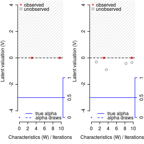
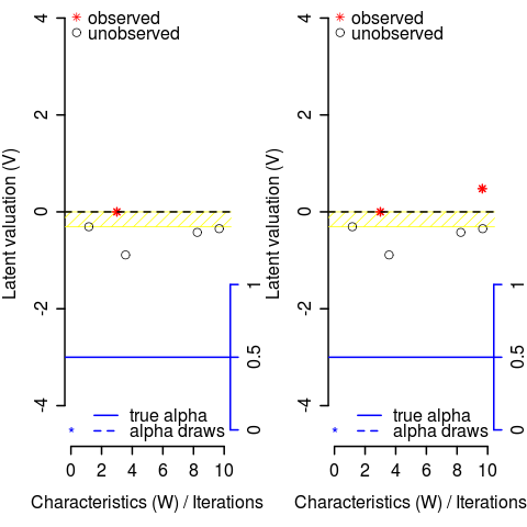
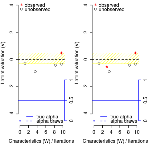
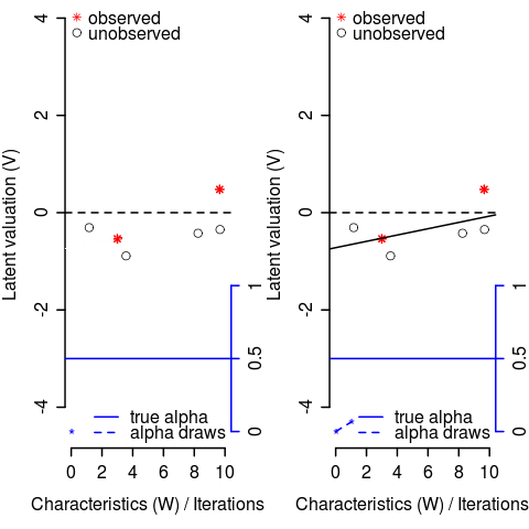
The Bayesian estimator uses the data augmentation approach (Albert and Chib, 1993, proposed by) that treats the latent outcome and valuation variables as nuissance parameters. The following four steps illustrate the first iteration of the estimator for the first-stage matching model.
0.B.1 Match valuations for unobserved groups
The algorithm starts by simulating the latent match valuations for unobserved groups conditional on the data and parameters. In the first iteration illustrated here, the slope parameter alpha (blue asterisk) and the match valuations of the equilibrium groups (red asterisks) are initially set to zero and match valuations for unobserved groups (black circles) are drawn from a normal distribution with mean zero. For the observed groups to be in equilibrium, the match valuation of the unobserved groups must be lower than the maximum equilibrium group valuation. The draws from the normal are therefore censored from above (gray shades).
0.B.2 Match valuations for first observed group
In the next step, the match valuation is drawn from a normal distribution with mean zero (conditional mean given by the dashed line). The equilibrium condition holds because the valuation of the second equilibrium group is larger than that of any non-equilibrium group (indicated by the yellow shades). Thus the valuation can be drawn from an uncensored normal.
0.B.3 Match valuations for second observed group
Same procedure as in step 2.
0.B.4 Alpha slope parameter
Fit a regression based on the given valuations and data (solid line) and draw alpha (dashed blue line) from a normal distribution with mean and standard deviation of the estimated slope parameter. Use the new alpha draw in the next iteration to simulate the latent match valuations, etc etc.
| 1. Match valuations for unobserved groups | 2. Match valuation for 1st observed group | |
| before. after. | before. after. | |
 |
 |
| 3. Match valuation for 2nd observed group | 4. Alpha slope parameter | |
| before. after. | before. after. | |
 |
 |
Affiliation
Thilo Klein
ZEW – Centre for European Economic Research
L7, 1
68161 Mannheim, Germany
E-mail: thilo.klein@zew.de
URL: https://klein.uk