Smoothing discrete data (I)
– using the smooth.discrete() function in the
mhsmm package
1 Introduction
The smooth.discrete() function provides a simple smoothing of a
time series of discrete values measured at equidistant times.
Under the hood of smooth.discrete() is a hidden Markov model.
More details – and an additional example – is provided in the vignette “Smoothing discrete data (II)”
2 Using smooth.discrete()
For example consider the data:
> y1 <- c(1,1,1,1,2,1,1,NA,1,1,2,1,1,1,2,1,1,1,1,1,2,2,2,2,1,2,2,2,1,2,2,2,1,1,1,1,1,1,1,1,2,2,2,1,1)
Calling smooth.discrete() on these data gives
> obj <- smooth.discrete(y1)
A 'smoothDiscrete' objectList of 4 $ s : num [1:45] 1 1 1 1 1 1 1 1 1 1 ... $ model :List of 9 ..- attr(*, "class")= chr "hmm" $ data :List of 3 $ initial:List of 3 - attr(*, "class")= chr "smoothDiscrete"NULL
The s slot of the object contains the smoothed values. We
illustrate the results in Figure 1.
> plot(y1, ylim=c(0.8,2))> addStates(obj$s)
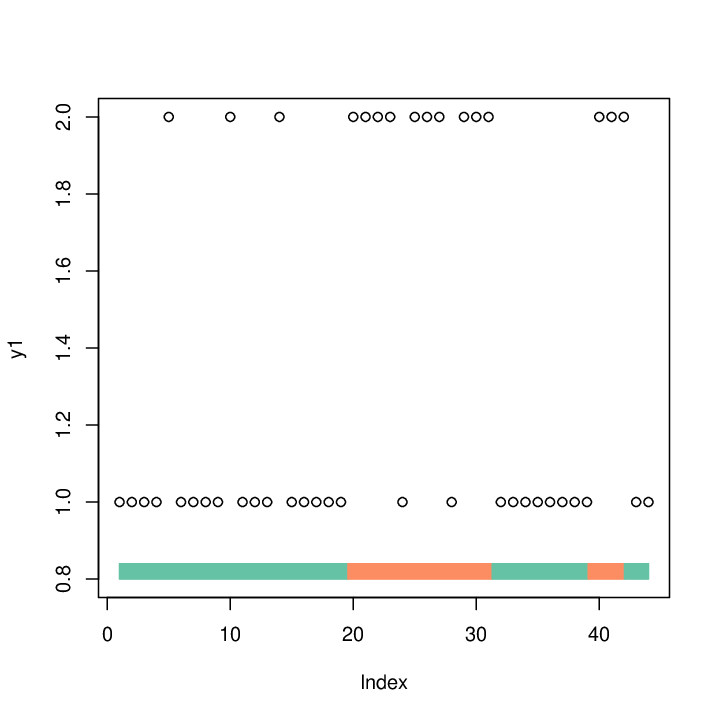
The smoothed sequence of states is by default the jointly most likely sequence of states as obtained by the Viterbi algorithm.
A smooth of a new time series is produced as
> y2 <- c(1,1,1,1,2,2,2,1,1,2,1,1,1,2,1,1,1,1,1,2,2,2,NA,1,1,1,2,2,1,2,2,2)> predict(obj,x=y2)
$s [1] 1 1 1 1 1 1 1 1 1 1 1 1 1 1 1 1 1 1 1 2 2 2 2 2 2 2 2 2 2 2 2 2$x [1] 1 1 1 1 2 2 2 1 1 2 1 1 1 2 1 1 1 1 1 2 2 2 NA 1 1[26] 1 2 2 1 2 2 2$N[1] 32$loglik[1] -24.53755attr(,"class")[1] "hsmm.data"
Here the smoothed values are in the s slot.
Again, the sequence is by default the jointly most likely
sequence of states.
The estimated parameters are:
> summary(obj)
init: 1 0transition: [,1] [,2][1,] 0.920 0.080[2,] 0.136 0.864emission:$pmf [,1] [,2][1,] 0.7925235 0.2147958[2,] 0.3418576 0.6443388
3 The arguments to smooth.discrete()
The arguments of smooth.discrete() are
> args(smooth.discrete)
function (y, init = NULL, trans = NULL, parms.emission = 0.5, method = "viterbi", details = 0, ...)NULL
- •
init is a vector of initial probabilities for the Markov chain. If init=NULL then the initial distribution is taken to be the relative frequencies in data, that is
> table(y1)/sum(table(y1))
y1 1 20.6363636 0.3636364
- •
trans is the transition matrix for the Markov chain. If trans=NULL then the transition matrix is derived from data as:
> ttt<-table(y1[-length(y1)],y1[-1])> ttt
1 2 1 19 7 2 7 9
> sweep(ttt, 1, rowSums(ttt), "/")
1 2 1 0.7307692 0.2692308 2 0.4375000 0.5625000
If trans is a vector (of numbers smaller than ) then these are taken to be the diagonal of the transition matrix and the off–diagonal elements are then, within each row, taken to be identical so that the rows sum to . Elements of trans are recycled so as to make the dimensions match. Under the hood, the matrix is created as, for example:
> createTransition(c(0.8,0.9),2)
[,1] [,2][1,] 0.8 0.2[2,] 0.1 0.9
- •
parms.emission is a matrix describing the conditional probabilities of the observed states given the latent states. If parms.emission is a vector then the matrix is created following the same scheme as for the transition matrix described above.
- •
The
methodargument is either"viterbi"(which produces the jointly most likely sequence of states). The alternative method issmoothedwhich produces the individually most likely states. - •
The dotted arguments are passed on the the
hmmfitfunction. For example, one may specify lock.transition=TRUE in which case the transition matrix is not estimated from data.