Linked Micromaps
1 Introduction
The R package micromap is used to create linked micromaps, which display statistical summaries associated with areal units, or polygons. Linked micromaps provide a means to simultaneously summarize and display both statistical and geographic distributions by linking statistical summaries to a series of small maps. The package contains functions, heavily dependent on the utilities of the ggplot2 package, which may be used to produce a row-oriented graph composed of different panels, or columns, of information. These panels at a minimum contain maps, a legend, and statistical summaries.
The key to using these functions is to have your data set up correctly. For a first example, we would like to display US state names, a graph illustrating their poverty level, a graph illustrating their percentage of college graduates, and a micromap indicating which states are being referenced. In order to do this, all we need is a table with state names and estimates of each of the two metrics we’re interested in. The dataset edpov included in the micromap package is in this form:
> library(micromap)> data("edPov")> head(edPov)
state ed pov region StateAbIL Illinois 26.1 10.7 MW ILIN Indiana 19.4 9.5 MW INIA Iowa 21.2 9.1 MW IAKS Kansas 25.8 9.9 MW KSMI Michigan 21.8 10.5 MW MIMN Minnesota 27.4 7.9 MW MN
Next, we need a table of polygons to map. We can use the create_map_table function to take a spatial object file and create a small efficient table in the form that the mmplot function can use or we can construct our table directly. In order to do this successfully our table must end up with 4 essential columns that must be named as follows: ID; coordsx; coordsy; and poly. The ID column is what links to the table of statistics. The poly column is used to identify state polygons for the same ID (otherwise R will connect all the vertices with some odd looking results). For this first example we will use the USstates included with the package and use create_map_table in order to get the data in the right format.
Some preliminary steps are usually required to use the create_map_table function. First, many spatial objects are quite detailed, far more detailed than what is needed for a micromap. The size and complexity of these files will drastically reduce the speed at which plots can be produced and, in some cases, overwhelm R with the amount of data being handled causing it to crash. One option for reducing shapefile complexity is to use a simplification function from the sf package which can be used to reduce the size and complexity of a spatial object. See Section 3,"Preparing data for use with the package", for more details and an example. The USstates data is very simple and therefore we will hold off discussion of the thinning function until later.
The second (and much simpler) step in successfully using the create_map_table function is assigning an explicit ID to each polygon. The data table associated with the spatial object must have an ID column (literally called ’ID’) to name each polygon. This is the column that will be used to link the information from the stat table to this built map table. With this in mind we can check the data table from our USstates file by using the following @data syntax. The "@" syntax refers to grabbing the data object stored in this slot of an sp spatial object. To examine the other slots of this shapefile one would use the slotNames() function.
> data("USstates")> head(USstates@data)
ST ST_NAME AREA_KM PERIM_KM0 AK Alaska 1506038.1 60260.6381 AL Alabama 133761.0 2354.6002 AR Arkansas 137733.7 2172.2083 AZ Arizona 295267.5 2395.4094 CA California 409603.3 5682.3045 CO Colorado 269599.9 2100.092
Since there is no ID column in this table we can insert a second argument into create_map_table identifying which column we would like to use as our ID. The ST column will be used in linking to our stats table so that will be used:
> statePolys <- create_map_table(USstates, IDcolumn="ST")> head(statePolys)
ID region poly coordsx coordsy hole plotorder plug1 AK 1 1 2 5 0 1 02 AK 1 1 7 10 0 1 03 AK 1 1 4 12 0 1 04 AK 1 1 7 15 0 1 05 AK 1 1 4 15 0 1 06 AK 1 1 4 17 0 1 0
From here we can create the draft micromap plot. To graph our poverty and college degree metrics we must specify the type of graph to be used. As of now, there are 5 types of graphs built in:
- •
Dot plots (with or without confidence limits)
- •
Bar plots (with or without confidence limits)
- •
Box summary
Additional graph types will be built and included as needed. Users can create and include new graph types as is explained later in section 5, “Creating a new panel/graph type”. The draft version of a micromap plot can be made with this code:
> mmplot(stat.data=edPov,map.data=statePolys,+ panel.types=c("labels", "dot","dot", "map"),+ panel.data=list("state","pov","ed", NA),+ ord.by="pov", grouping=5,+ median.row=T,+ map.link=c("StateAb","ID"),+ print.file="fig1.jpeg",print.res=100+ )
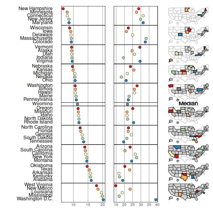
A full explanation of all the function arguments is provided below but 3 things should be made clear here:
- •
panel.data is list of lists to specify which columns of the stat.data table to use in filling out the panels. For a panel needing multiple columns you would enter a sublist. There needs to be an entry for every panel even when specific data from the stat table isn’t supplied by the user. As you can see here, the map panel has an NA entry. These entries cannot be left out. Note: The order of the entries in panel.data and panel.types must coincide. If we want to rearrange the order of the panels, the entries of both panel.data and panel.types need to be rearranged.
- •
map.link is a vector specifying which column from the stat table matches the respective column from the map table. In this example the StateAb column from the stat table matches each data line to its associated polygons in the map table labeled by matching entries in that table’s ID column. Note that the StateAB column and the ID column have to be of the same case. Here both columns are uppercase.
- •
Setting median.row=TRUE will insert a median row. As is noted below, this will override the default to force the x and y axis coordinates to stay respective to each other which will probably cause distortion in the maps being presented. Adjusting panel.width should be used to manually correct this. If median.row is specified with an even number of polygons then the median is simply the average of the values of the n/2 and (n/2)+1 polygons. As that median value will not correspond to an observed data value and polygon then that median value is plotted on the statistical panel, but no label or polygon are assigned to that symbol.
This initial call will rarely result in high quality, final looking results. From here we can make notes on what adjustments would make this look better. We are attempting to replicate a figure created by Dan Carr http://mason.gmu.edu/~dcarr/ and so we must make some adjustments.
As with most R functions, a few plot wide adjustments can be made by simply adding in extra arguments in the function call (such as plot.height, colors, and inactive.fill in this example). To adjust the individual panels, however, we must make a list of lists specifying which panel we are adjusting and then which attributes we would like to modify.
To make this more intuitive here is a quick and simple example. Suppose we just want to change the text alignment in panel 1 and the graph background colors in panels 2 and 3. First we make a list for each of these panels specifying the changes we would like to make with the first entry of each list specifying which panel is to be altered:
> list(1, align="left")> list(2, graph.bgcolor="lightgray")> list(3, graph.bgcolor="lightgray")Now we compile these lists into a list of lists:
> list(list(1, align="left"), list(2, graph.bgcolor="lightgray"),+ list(3, graph.bgcolor="lightgray"))
Now we can just add:
panel.att= list(list(1, align="left"), list(2, graph.bgcolor="lightgray"), list(3,graph.bgcolor="lightgray"))
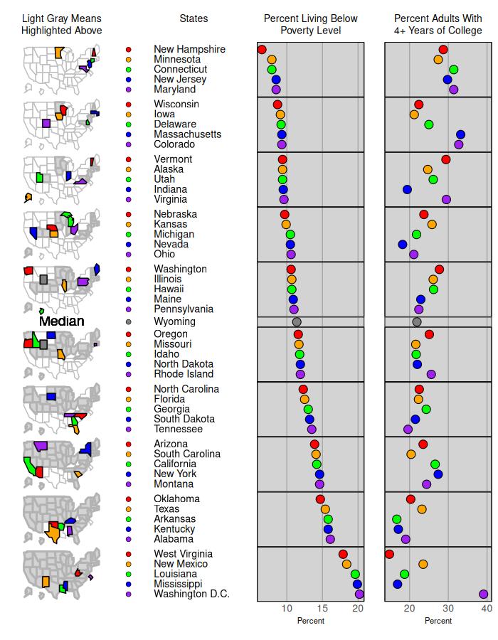
to our mmplot function call and see the changes. We have a lot more changes to make, though, so we might as well implement all of them at once. The following code is used to make the graph below in Figure 2:
> mmplot(stat.data=edPov, map.data=statePolys,+ panel.types=c("labels", "dot", "dot","map"),+ panel.data=list("state","pov","ed", NA),+ ord.by="pov", grouping=5,+ median.row=T,+ map.link=c("StateAb","ID"),+ plot.height=9,+ colors=c("red","orange","green","blue","purple"),+ panel.att=list(list(1, header="States",+ panel.width=.8,+ align="left", text.size=.9),+ list(2, header="Percent Living Below \n Poverty Level",+ graph.bgcolor="lightgray", point.size=1.5,+ xaxis.ticks=list(10,15,20), xaxis.labels=list(10,15,20),+ xaxis.title="Percent"),+ list(3, header="Percent Adults With\n4+ Years of College",+ graph.bgcolor="lightgray", point.size=1.5,+ xaxis.ticks=list(20,30,40), xaxis.labels=list(20,30,40),+ xaxis.title="Percent"),+ list(4, header="Light Gray Means\nHighlighted Above",+ inactive.fill="lightgray",+ inactive.border.color=gray(.7), inactive.border.size=2,+ panel.width=.8)), print.file="fig2.jpeg",+ print.res=100)
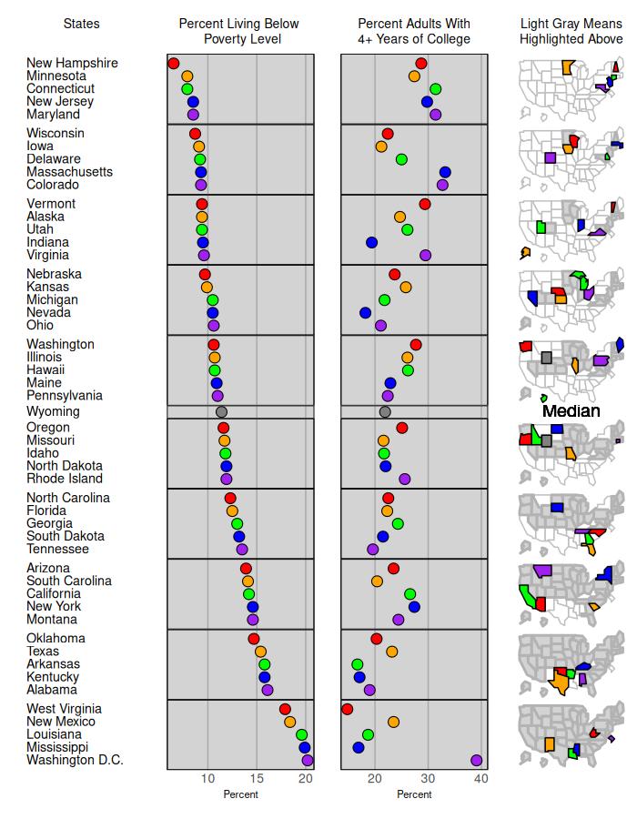
This seems pretty good. Note “\n” inserts a carriage return in the header. Actual carriage returns have the same effect but should not be used as this will result in mmplot being unable to properly align panels, e.g. use:
“…header="Percent Living Below \n Poverty Level"…”
not
“…header="Percent Living Below
Poverty Level"…”
We have two options for storing this final figure. In the mmplot function call we can add a line to the final list of panel attributes specifying a filename (and resolution if desired) as follows:
“mmplot(stat.data=edPov,…,print.file=’myFigure.tiff’, print.res=100)”
The “.tiff” tells the mmplot function that a tiff file is requested. Jpeg, jpg, png, ps, and eps files may also be produced in a similar manner. The other option is to store our function output in an R object as we build it. When we have results
we are satisfied with we can use the printmmplot function to print it out:
myPlot <- mmplot(stat.data=edPov,…)
print(myPlot, name=“myFigure.tiff”, res=300)
2 Quick Plotting Tips
Quick tips for making higher quality figures with the mmplot function:
- •
Panel widths will almost certainly need to be adjusted in order to have the text correctly fit across the panel. Text in the labels and ranks panels are defaulted to fit vertically correctly. If text is overlapping vertically, it may be because not enough vertical space is being provided on the plot. Adjusting plot.height (defaults to 7) and plot.pGrp.spacing (defaults to 1) can, and should, be used to correct this.
- •
Adjusting right and left panel margins are perhaps the most useful tool in making a plot look nice. Panels are printed out from left to right and many times a panel will overlap its preceding neighbor; therefore bringing in the left margin by setting left.margin=-.5 or even left.margin=-1 can be very helpful in clearing out white space. For neighboring panels (such as the poverty and education panels in the example) adjusting the left panel’s right margin and the right panel’s left margin can cause them to share a border thus appearing attached.
- •
As noted elsewhere, the micromaps are set to have the x and y axis coordinates set respective to each other. This causes quite a few unintended consequences, one of which is micromap “shrinkage” if the panel.width is not wide enough. If your maps look too small at first, expanding the panel width will probably enlarge your graph quite a bit.
- •
Also, due to an artifact (some might call it a bug) in ggplot2, this coordinate “respectivity” in the micromaps goes away when adding a median row. Therefore, one should be careful in such situations and take care in setting the panel width of the map panel to correct any distortion that may present itself.
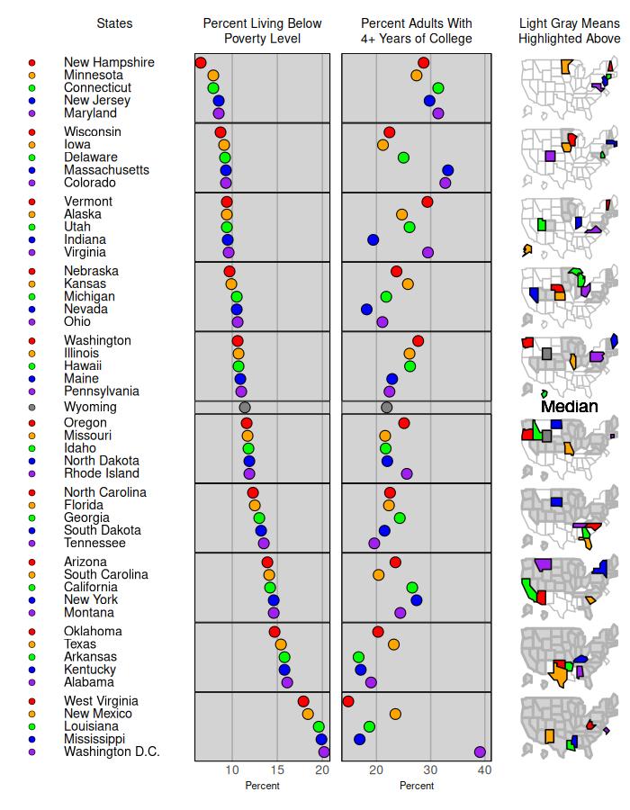
We can illustrate these options by adding to our example. Suppose we wish to add a series of color coded bullets in front of our state names in the original poverty and education micromap. We can do this by specifying the dot_legend panel.type. This now gives us five panel types.
> mmplot(stat.data=edPov,map.data=statePolys,+ panel.types=c("dot_legend","labels","dot","dot","map"),+ panel.data=list(NA,"state","pov","ed",NA),+ map.link=c("StateAb","ID"),+ ord.by="pov",+ grouping=5,+ median.row=T,+ plot.height=9,+ colors=c("red","orange","green","blue","purple"),+ panel.att=list(list(1, point.type=20, point.border=TRUE),+ list(2, header="States", panel.width=.8,+ align="left", text.size=.9),+ list(3, header="Percent Living Below\nPoverty Level",+ graph.bgcolor="lightgray", point.size=1.5,+ xaxis.ticks=list(10,15,20), xaxis.labels=list(10,15,20),+ xaxis.title="Percent"),+ list(4, header="Percent Adults With\n4+ Years of College",+ graph.bgcolor="lightgray", point.size=1.5,+ xaxis.ticks=list(20,30,40), xaxis.labels=list(20,30,40),+ xaxis.title="Percent", left.margin=-.8, right.margin=0),+ list(5, header="Light Gray Means\nHighlighted Above",+ inactive.fill="lightgray",+ inactive.border.color=gray(.7), inactive.border.size=2,+ panel.width=.8)),+ print.file="fig3.jpeg",print.res=100)
Note the correspondence between the panel.types and panel.data statements. The panel.data statement refers to the data from the statistical data frame edPov. The first "dot_legend" in panel.types corresponds to the "NA" as no statistcal data are being referenced, the "labels" corresponds to the "state" column, the second "dot" corresponds to the poverty column, and the third "dot" corresponds to the education column. The last panel.type, "map" corresponds to "NA" in the panel.data list as there is no map data in the edPov data frame. The map data is associated with the statePolys data frame. Also, note that the addition of the dots before the state names increased the number of panels displayed in the linked micromap to five so the panel.att statement contains five lists now.
A final option that we can illustrate is that we can easily rearrange the panels by changing the order of the panel.types and panel.data by re-numbering the panel attributes section. We now move the maps to the first panel.
> mmplot(stat.data=edPov,map.data=statePolys,+ panel.types=c("map","dot_legend","labels","dot","dot"),+ panel.data=list(NA,NA,"state","pov","ed"),+ map.link=c("StateAb","ID"),+ ord.by="pov",+ grouping=5,+ median.row=T,+ plot.height=9,+ colors=c("red","orange","green","blue","purple"),+ panel.att=list(list(2, point.type=20,+ point.border=TRUE),+ list(3, header="States", panel.width=.8,+ align="left", text.size=.9),+ list(4, header="Percent Living Below\nPoverty Level",+ graph.bgcolor="lightgray", point.size=1.5,+ xaxis.ticks=list(10,15,20), xaxis.labels=list(10,15,20),+ xaxis.title="Percent"),+ list(5, header="Percent Adults With\n4+ Years of College",+ graph.bgcolor="lightgray", point.size=1.5,+ xaxis.ticks=list(20,30,40), xaxis.labels=list(20,30,40),+ xaxis.title="Percent"),+ list(1, header="Light Gray Means\nHighlighted Above",+ inactive.fill="lightgray",+ inactive.border.color=gray(.7), inactive.border.size=2,+ panel.width=.8)),+ print.file="fig4.jpeg",print.res=100)
3 Preparing data for use with the package
Example Steps for simplifying spatial polygons in a spatial data set for the mmplot function:
Users can download an example shapefile. We will use level 3 ecoregions of Texas as an example (located here):
https://www.epa.gov/eco-research/level-iii-and-iv-ecoregions-state
We will look at two approaches to simplifying spatial polygons for use in micromaps —one using GIS software such as ESRI ArcMap and the other entirely in R.
Method for simplifying polygons using simplification in GIS software such as ArcMap:
- •
Read the shapefile into R from your working directory
File > Add Data > navigate to where you downloaded file
- •
Open the Simplify Polygon tool in ArcToolbox
Generalization > Simplify Polygon
- •
Choose simplification algorithm, maximum allowable offset, and minimum area. Point remove is quick, bend simplify can take longer but gives more aesthetically pleasing results
Simplification Algorithm: POINT_REMOVE
Maximum Allowable Offset: 1000 Meters
Minimum Area: .001
Handling Topological Errors: RESOLVE_ERRORS
- •
Read resulting shapefile into R using
st_read(usesst_readfromsf, loaded with themicromappackage):> txeco <- st_read(“tx_eco_l3ṡhp”)
- •
Convert the imported shapefile to a spatial dataframe using
as_Spatialfromsf:> txeco <- as_Spatial(txeco)
- •
Create an ID column in your spatial dataframe for the
create_map_tablefunction> txeco$ID <- txeco$US_L3CODE
Method two is to simplify polygons within R , and this can be done using the st_simplify function from the sf package.
Steps for simplifying very large spatial data:
For very large data you need to take extra steps to get manageable spatial data for use in linked micromaps. We will use level 3 ecoregions for the conterminous US as an example. Note that these are one example of steps that work, other combinations of steps could possibly work better for other data —the point is to get rid of very small features and simplify line work as much as possible.
First we’ll download level 3 ecoregions for the US (located here):
https://www.epa.gov/eco-research/level-iii-and-iv-ecoregions-continental-united-states
In ArcMap:
- •
To get rid of state boundaries, first open the Dissolve tool in the Generalization toolbox:
Generalization > Dissolve
- •
Simplify newly created feature using the Simplify Polygon tool:
Cartography Tools > Generalization > Simplify Polygon
Choose simplification algorithm = Bend Simplify, Reference Baseline 100 kilometers, minimum area 100 square kilometers, and handling toplogical errors = resolve errors
- •
Now simplify features you just created again, but using a different simplification algorithm:
Open Simplify Polygon tool
Choose simplification algorithm = Point Remove, Maximum allowable offset 10,000 meters, minimum area 10,000 square meters, and handling toplogical errors = resolve errors
This will create a sufficiently simplified shapefile to use with the mmplot function.
In R:
Simplification methods to try in R are available using the sf package, specifically the st_simplify function.
- •
Load the shapefile using
st_readfromsf:> txeco <- st_read(“tx_eco_l3.shp”)
- •
Simplify using
st_simplify, set the options to preserve topology and the desired tolerance (in units of the CRS, meters in this case):> txecosimp <- st_simplify(txeco, preserveTopology = T, dTolerance = 1000)
- •
Convert the simplified dataset to a spatial dataframe using
as_Spatialfromsf, as needed:> txecosimp <- as_Spatial(txecosimp)
Other simplification approaches using open source or free tools include the online tool MapShaper available here:
https://mapshaper.org/. Both polygon simplification as well as line smoothing (Bezier curves for instance)
can be implemented as well in Quantum GIS via the ’Generalizer’ plugin, and in PostGIS the Douglas-Peucker algorithm is implemented with ’simplify’.
For further reading on polygon simplification, we refer users to the following papers:
Douglas, D. and Peucker, T. (1973). Algorithms for the reduction of the number of points required to represent a digitized line or its caricature. The Canadian Cartographer 10(2). 112-122.
Harrower, M. and Bloch, M. (2006). MapShaper.org: A Map Generalization Web Service. IEE Computer Graphics and Applications 26(4). 22-27.
Mansouryar, M. and Hedayati, A. (2012). Smoothing Via Iterative Averaging (SIA) A Basic Techniqu for Line Smoothing. International Journal of Computer and Electrical Engineering 4(3), 307-311.
Technical paper, ESRI, "Automation of Map Generalization: The Cutting-Edge Technology," 1996. It can be found in the White Papers section of ArcOnline at this Internet address: https://content.esri.com/support/whitepapers/ao_/mapgen.pdf
4 Full List of Adjustable Attributes
- •
Attribute arguments recognized by the mmplot function:
- •
cat - category column within stats table for a categorization type linked micromap.
- •
colors - the color palette used within each perceptual group. (e.g. brewer.pal(5, "Spectral")).
- •
grouping (required)- the number of lines per perceptual group. E.g. simply entering “5” will put 5 lines in each perceptual group or you can enter c(5,6,5,4) to have disproportionate numbers of lines in each group.
- •
map.data (required) - data table likely created by the create_map_table function applied to a spatial polygon data frame.
- •
map.link (required, but see section 7) - a vector specifying which column from the stat table matches which column from the map table respectively (e.g. “c(“StateAb”, “ID”))”. The two columns must be of the same case.
- •
median.color - if median.row is specified, then the user can specify the color for the median symbol, such as median.color="black".
- •
median.row - specifies whether a median row should be included. If an odd number of data lines are supplied a data line itself will be used as the median; otherwise median entries will be calculated from the supplied data. Note that without a median row maps are forced into proper size. However, an artifact in
ggplot2removes this feature when a median row is added and so a user must use the panel.width argument (and left.margin/right.margin panel attribute) for the map panel so that panel that does not have distorted coordinates. (The default setting is FALSE) - •
median.text.color - the default is median.text.color=’black’. Other colors can be specified to change the color of the word Median plotted when median.row=TRUE.
- •
median.text.label - the default is median.text.label=’Median’ when median.row=TRUE.
- •
median.text.size - the default is median.text.size=1 when median.row=TRUE. As with all defaults set to 1, any change from default will magnify the default size by a factor. For example, median.text.size=.5 will print the word "Median" half as big as the default size.
- •
ord.by, grp.by (required) - ord.by specifies the stats.data column to be ranked for the ordering of the figure. See related rev.ord. grp.by is used for grouped plots in order to specify which data table column to sort the figure by.
- •
panel.att - a list of panel specific attributes to be altered (described in more detail below).
- •
panel.data (required) - a list of lists to specify which columns of the stat.data table to use in filling out the panels. For a panel needing multiple columns you enter a sublist. For example, the dot_cl requires a sublist that includes three column names from the statistics data frame. One column name identifies the summary statistics, and the other two column names identify the lower and upper confidence bounds. There needs to be an entry for every panel even when specific data from the stat table isn’t supplied by the user. That is to say map and rank panels (as well as user created panel types) should have NAs. e.g. panel.data=list(“State”, list(“Estimate”, “Lower.Bound”, “Upper.Bound”), NA).
- •
panel.types (required) - a vector specifying the panels of the plot. Note: each “panel.type” (e.g. “map”, “labels”, “dot_cl”, etc.) is the name of a function that will be called to create that panel. Nine total types are available: “map”, “labels”, “dot”, “dot_cl” (dotplots with confidence limits), ‘’dot_legend’‘, ‘’bar’‘, ‘’bar_cl’‘ (barplots with confidence limits), “box_summary”, and “ranks”. A user can create a new panel type (e.g. “new.graph.type”) and the mmplot function will automatically go look for and call that function just by changing the entry here. See the section “Creating a New Panel Type”.
- •
plot.footer - not implemented yet.
- •
plot.footer.size - not implemented yet.
- •
plot.footer.color - not implemented yet.
- •
plot.grp.spacing - the verticle spacing between groups measured in lines. Defaults to 1.
- •
plot.pGrp.spacing - the spacing between perceptual groups. “1”, the default, implies standard spacing.
- •
plot.header - not implemented yet.
- •
plot.header.size - not implemented yet.
- •
plot.header.color - not implemented yet.
- •
plot.height - the height of the plot window.
- •
plot.width - the width of the plot window. (Defaults to 7)
- •
print.file - the full file name (i.e. including extension) to save the resulting figure. The extension tells the mmplot function which type of printing function to run. Tiff, png ,jpeg, .jpg, .ps, or .eps are all recognized.
- •
print.res - the resolution desired for the resulting file.
- •
rev.ord - reverse the order for ranking the plot.
- •
stat.data (required, but see section 7) - data table of statistic.
- •
vertical.align - the default is vertical.align="top" specifying that the rows within a perceptual group are aligned at the top. Specifying vertical.align="center" will center align the rows within a perceptual group, which is useful when perceptual groups do not contain the same number of rows, such as group=c(5,5,4,4,5,5)
- •
Attribute arguments applied to the panels:
- •
panel.att - is a list object (simply referred to as “a” throughout the function) which contains a sublist of specifications for each panel. Some attributes are standard for all panel types (e.g. header, graph color, etc.), while other options are only available to alter for certain panels (bar size, point type, etc.). If a user tries to alter a panel specific attribute that isn’t recognized (e.g. bar size on a dot plot), it is ignored and a warning is printed.
Standard Attributes
- •
graph.bgcolor -the background color within any graphs being drawn.
- •
graph.border.color - alters the border color on graphs. Note this can be used to hide borders on graphs by setting it equal to white or whatever the specified panel background color is. Defaults to “Black” on graphs. No borders are shown on maps, labels and ranks.
- •
graph.grid.major - a boolean variable stating whether major grid lines should appear in the graph. (T/F or 0/1 should both work). The defaults is “TRUE” for graphs, and “FALSE” for all other panels.
- •
graph.grid.minor - see above.
- •
panel.att - a list of panel specific attributes. These are to be entered as a list of lists, with the first entry of each sublist specifying with panel’s attributes are being altered: For example panel.att=list(list(1, …),list(2, …),…, list(n, …)) The following attributes can be specified for each list.
- •
left.margin, right.margin - set panel specific panel margins individually.
- •
panel.bgcolor - the back ground color in each panel.
- •
panel.footer - not implemented yet.
- •
panel.footer.size - not implemented yet.
- •
panel.footer.color - not implemented yet.
- •
panel.header - a title for the whole panel.
- •
panel.header.size - size relative to default. All panels should have the same size header to keep proper alignment between panels. If a user has specified unequal header sizes between panels, the function will return a warning.
- •
panel.header.color - not implemented yet.
- •
panel.width - this is the relative panel width compared to the other panels.
- •
xaxis.color - the color of the x axis line.
- •
xaxis.labels - this is a list or vector of text to be written at each tick mark. Note: if these are being explicitly specified then xaxis.ticks must be explicitly specified as well. e.g. xaxis.labels=list(500,1000,1500,2000)
- •
xaxis.labels.angle - rotates the labels on the x axis. The default xaxis.labels.angle=0 has the labels horizontally arranged; whereas xaxis.labels.angle=90 orients the labels vertically.
- •
xaxis.labels.size - controls the size of of the labels under the x axis of the panels by specifying, for example, xaxis.labels.size=c(1.5). All x axis labels will be sized the same across the panels.
- •
xaxis.line.display - a boolean variable stating whether the line of the x axis should appear on the graph. (T/F or 0/1 should both work). This defaults to “FALSE”on maps, labels and ranks panel types so no x axis line is displayed for those panels.
- •
xaxis.text.display - a boolean variable indicating whether text should be displayed on the x axis. This is the text associated with each tick, not the axis title. For the panel types of maps, labels, and ranks the default is set to “FALSE”.
- •
xaxis.ticks - this is a list or vector of points at which ticks should be drawn on the x axis. e.g. xaxis.ticks=list(500,1000,1500,2000)
- •
xaxis.ticks.display - a boolean variable stating whether the axis ticks should appear on the x axis. (T/F or 0/1 should both work) Defaults to "FALSE" on all graphs.
- •
xaxis.title - specifies what the x axis should be labeled. The default is for to no axis label.
- •
yaxis.labels - see description for xaxis.labels.
- •
yaxis.line.display - see description for xaxis.line.display.
- •
yaxis.text.display - see description for xaxis.text.display.
- •
yaxis.ticks - see description for xaxis.ticks.
- •
yaxis.ticks.display - see description for xaxis.ticks.display.
- •
yaxis.title - see description for xaxis.title.
Attributes for Specific Panel Types labels:
- •
align - horizontal alignment for labels with alignment options of “center”, “left”, “right’.
- •
text.size - relative to default size.
ranks:
- •
align - horizontal alignment for ranks with alignment options of “center”, “left”, “right”.
- •
text.size - relative to default size.
dot_legend:
- •
point.border - by default a black border will be placed around dots. To correct this, set this option to FALSE.
- •
point.size - size relative to default.
- •
point.type - the pch specification for points contained in a graph.
dot:
- •
add.line - add a line at some specified x coordinate.
- •
add.line.col - specify color.
- •
add.line.typ - specify type**.
- •
connected.dots - set equal “TRUE” makes a line connecting the dots within each perceptual group of a dot plot.
- •
connected.col - color of the connecting line, such as “gray(.6)”.
- •
connected.typ - specify line type, such as = “solid”, for the connecting line.
- •
connected.size - specify the size of the line type for the connecting line.
- •
median.line - add a line at the calculated median.
- •
median.line.col - specify line color.
- •
median.line.typ - specify type**.
- •
point.border - by default a black border will be placed around dots. To correct this, set this option to FALSE.
- •
point.size - size relative to default.
- •
point.type - the pch specification for points contained in a graph.
dot_cl: requires a sublist identifying that statistics column and the two columns containing the lower and upper confidcence bounds from the statistics data frame.
- •
add.line - add a line at some specified x coordinate.
- •
add.line.col - specify color.
- •
add.line.typ - specify type**.
- •
line.width - thickness of confidence bands relative to default.
- •
median.line - add a line at the calculated median.
- •
median.line.col - specify line color.
- •
median.line.typ - specify type**.
- •
point.border - by default a black border will be placed around dots. To correct this, set this option to FALSE.
- •
point.size - size relative to default.
- •
point.type - the pch specification for points contained in a graph.
bar:
- •
add.line - add a line at some specified x coordinate.
- •
add.line.col - specify color.
- •
add.line.typ - specify type**.
- •
graph.bar.size - relative to default size
- •
median.line - add a line at the calculated median.
- •
median.line.col - specify line color.
- •
median.line.typ - specify type**.
bar_cl: see description of dot_cl sublist
- •
add.line - add a line at some specified x coordinate.
- •
add.line.col - specify color.
- •
add.line.typ - specify type**.
- •
graph.bar.size - relative to default size
- •
median.line - add a line at the calculated median.
- •
median.line.col - specify line color.
- •
median.line.typ - specify type**.
box_summary: requires a sublist identifying for a five-number summary the columns containing the minimum, first quartile, median, third quarterile, and maximum from the statistics data frame.
- •
add.line - add a line at some specified x coordinate.
- •
add.line.col - specify color.
- •
add.line.typ - specify type**.
- •
graph.bar.size - relative to default size
- •
median.line - add a line at the calculated median.
- •
median.line.col - specify line color.
- •
median.line.typ - specify type**.
map:
- •
map.all - by default, the mmplot function will only plot the polygons associated with data in the stats table. Setting “map.all=T” will tell it to show all the polygons from the map table regardless of whether the polygons have data associated with the stats table. Setting “map.all=F” eliminates polygons from the map that do not have data associated with the stats table.
- •
fill.regions="aggregate" is the default and creates the standard micromap in which polygons in a previous perceptual group are shaded or filled in subsequent perceptual groups. The fill.regions=“aggregate” proceeds from the top perceptual group to the bottom perceptual group by sequentially filling the polygons that have already been displayed. Arguments typically used when fill.regions=“aggregate” is specified include:
- •
active.border.color - specifies the border color of the polygons that are linked to the statistical summaries being displayed in that row’s perceptual group. The default is active.border.color=“black”.
- •
active.border.size - specifies the size of the line around the border of the polygons that are linked to the statistical summaries being displayed in that row’s perceptual group. The default is active.border.size=1.
- •
inactive.fill - “lightgray” is the default, and inactive polygons are those polygons that were displayed in a previous perceptual group.
- •
inactive.border.color - gray(.25) is the default.
- •
inactive.border.size - 1 is the default.
- •
fill.regions =“two ended” is typically used along with the median.row=T statement to indicate which polygons are above or below the median value of the variable specified in the ord.by= statement. With fill.regions=“two ended”, the active and inactive arguments previously described are only applied to the subset of polygons that are above the median or the subset below the median.
- •
fill.regions = "with data" simply applies a fill to all the polygons not being displayed in a specific row of a perceptual group. These polygons do have statistical data that will be displayed in a later perceptual group. Additional arguments used with fill.regons=“with data” include:
- •
withdata.fill - “white” is the default.
- •
withdata.border.color - “gray(.75)” is the default.
- •
withdata.border.size - “1” is the default.
Two other arguments can be applied to the map panel for two situations when a user wants to display polygons on the map, but those polygons are not included in the statistics data table. Such “no data” polygons will never be included in a perceptual group. In the first situation, fill, border color, and border size arguments are used so that the individual polyons that have no statistical data are displayed. These arguments are:
- •
nodata.fill - “white” is the default.
- •
nodata.border.color - “gray(.75)” is the default.
- •
nodata.border.size - “1” is the default.
In the second situation, the user does not want to display the individual polygons of the no data polygons. For example, forty-seven states have statistical summary data on a public health variable, but Alabama, Georgia, and Florida do not. With the “outerhull” arguments, the three individual polygons of Alabam, Georgia, and Florida are not displayed in the map, but only their exterior border outline, or outer hull, are displayed; whereas the polygons for the forty-seven other states are displayed on the map panel.
- •
outer.hull - setting equalt to “TRUE” draws only the outer.hull.
- •
outer.hull.color - “black” is the default.
- •
outer.hull.size - is the size of the line, with the default of “1”.
***Here is a helpful site for line types: http://www.cookbook-r.com/Graphs/Shapes_and_line_types/ See the section “Creating a New Panel Type” on how to specify other attributes.
5 Creating a new panel type
Note: A general understanding of ggplot2 is needed and assumed throughout this section
Now let’s say we would like to illustrate the change in lung cancer rates using arrows on a graph. We can build our own graph type by creating our own graphing function; we’ll call it arrow.plot.build. The mmplot function sends all
graphing functions the same arguments (in this order): the panel ggplot2 object being worked on; the number of the panel; the stats data table; and the attributes list (this is a little involved so we won’t get into it until a little later).
(Note: the panel number tells you which sublist in the attribute list to work with). To start, let’s get our data and store it in a new object:
> data(lungMort)> myStats <- lungMort> head(myStats)
StateAb Rate_95 Count_95 Lower_95 Upper_95 Pop_95AK AK 50.0 298 44.2 56.3 1089123AL AL 40.2 4095 39.0 41.4 8124753AR AR 43.8 3079 42.3 45.4 5479988AZ AZ 38.4 4794 37.3 39.5 10557561CA CA 41.5 26931 41.0 42.0 64354973CO CO 31.5 2723 30.3 32.7 9245273 StdErr_95 Rate_00 Count_00 Lower_00 Upper_00 Pop_00AK 3.1 46.8 350 41.8 52.2 1122525AL 0.6 43.4 4630 42.2 44.7 8245919AR 0.8 48.3 3568 46.7 49.9 5661547AZ 0.6 38.5 5482 37.4 39.5 12066024CA 0.3 39.2 27406 38.7 39.6 68478617CO 0.6 33.9 3265 32.7 35.1 10159130 StdErr_00 StateAK 2.6 AlaskaAL 0.6 AlabamaAR 0.8 ArkansasAZ 0.5 ArizonaCA 0.2 CaliforniaCO 0.6 Colorado
For the time being, we’ll also remove Washington D.C. so that we have nice even grouping numbers and can momentarily avoid the median row topic.
> myStats <- subset(myStats, !StateAb=="DC")
The data table that will actually be passed into our graphing function once we implement it into the function is not exactly like our stats table. Before constructing the panels, the mmplot function adds the extra columns "rank",
"median", "color", "pGrp" and "pGrpOrd" that specify, respectively, the overall order to plot the information, whether the row should be seperated as a median, the color from the color list to use, the perceptual group each table
entry belongs to and the order in each perceptual group of each entry. These columns are added using a built-in function called create_DF_rank. The syntax for this function is: create_DF_rank (data, ord.by, group). We
need these columns to know the nature of what we are working with in order to build our new graph type.
For now, we can assume groups of 5 will look good and we will want our table ordered by the rate from 2000. To create a new table with these columns file we run:
> myNewStats <- create_DF_rank(myStats, ord.by="Rate_00", group=5)> head(myNewStats)
pGrp StateAb Rate_95 Count_95 Lower_95 Upper_95 Pop_951 1 UT 17.6 685 16.3 18.9 50366382 1 ND 30.6 574 28.1 33.3 15278533 1 NM 31.8 1293 30.1 33.6 38994554 1 SD 30.5 659 28.2 33.1 17100035 1 CO 31.5 2723 30.3 32.7 92452736 2 ID 33.0 981 31.0 35.2 2976963 StdErr_95 Rate_00 Count_00 Lower_00 Upper_00 Pop_001 0.7 16.9 738 15.7 18.2 54884752 1.3 31.4 608 28.9 34.1 14809153 0.9 31.5 1420 29.9 33.2 40381634 1.2 32.9 736 30.5 35.5 17166835 0.6 33.9 3265 32.7 35.1 101591306 1.1 35.0 1158 33.0 37.1 3230513 StdErr_00 State rank median addOrd pGrpRank1 0.6 Utah 1 FALSE 0 12 1.3 North Dakota 2 FALSE 0 23 0.8 New Mexico 3 FALSE 0 34 1.2 South Dakota 4 FALSE 0 45 0.6 Colorado 5 FALSE 0 56 1.0 Idaho 6 FALSE 0 1 pGrpOrd color1 1 12 2 23 3 34 4 45 5 56 1 1
Now, to build our new graphing function, we have 4 basic steps to go through:
- 1.
create the general graph’s structure
- 2.
generalize the inputs
- 3.
integrate it with the mmplot function
- 4.
enable user customization if desired
Step 1: First we use ggplot2 to create the general structure of the graphs as we would like to see them. We can use geom_segment function in ggplot2 to make arrows. On our graph we would like an arrow starting at the 1995 rate extending to the 2000 rate so these columns will obviously be used for our "x" and "xend" parameters. The y coordinates can be inferred from the "pGrpOrd" column which has been created for just this purpose. Setting both the "y" and "yend" parameters equal to "pGrpOrd" should result in a flat arrow for each state, descending down our graph in an order which will match our label column as well as any other graphs being presented.
First, we can use the "color" column (which is calculated in create.DF.rank based on the pGrpOrd column) to vary the color of arrows within each perceptual group. Second, for various portions of the mmplot function code, we must
use facet_grid instead of facet_wrap.
> library(ggplot2)> library(grid)> ### ggplot2 code:> ggplot(myNewStats) ++ geom_segment(aes(x=Rate_95, y=-pGrpOrd,+ xend=Rate_00, yend=-pGrpOrd, colour=factor(color)),+ arrow=arrow(length=unit(0.1,"cm"))) ++ facet_grid(pGrp~., scales="free_y") ++ scale_colour_manual(values=c("red","orange","green","blue","purple"),+ guide="none")> ggsave(file="fig5.jpeg", dpi=300)
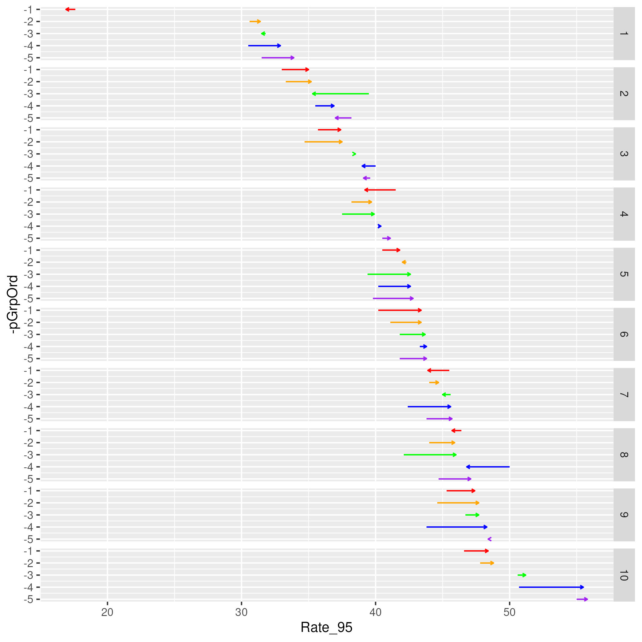
Step 2: This graph in Figure 5 looks like it is in the basic form we need. Good initial start but we need to change our x coordinate columns and color palette from being hard coded to being user specified. As noted earlier, the mmplot function provides the panel object, the panel number, the stats data table and the attribute list. It is this attributes list through which the color and data specifications are going to be provided to the function. Without delving too far into the details of this list just yet, we can take for granted that the user
specified color palette will be stored in the colors slot in the plot
section of the object and the names of our data columns will be stored in the panel.data slot of one of the panel sections; the panel number tells us which panel section to look in.
In writing our function we can refer to the panel object, the panel number, stats table and the attribute list however we like. We’ve already been referring to the data table as myNewStats so, along those same lines, let’s call the other items myPanel, myNumber, and myAtts respectively. In the next section we will start referring to myAtts and myNumber so it is helpful to set up a fake list and fake number to work with while we build our function that we can work with to test our code as we go along. The sample.att function will provide this list for us and we will simply set myNumber equal to 1.
> myAtts <- sample_att()> myNumber <- 1
This is just a dummy attribute list for now so we need to overwrite its entries with our specifications from above so that we can continue to test and have everything work as expected:
> myAtts$colors <- c("red","orange","green","blue","purple")> myAtts[[myNumber]]$panel.data <- c("Rate_95","Rate_00")
We will pull out our color list and panel column list into variables called myColors and myColumns. This means myColumns will be a vector with the myColumns[1] referring to the start points and myColumns[2] referring to the end points of our arrows. The code to pull these items out of the attributes list will look like this:
> myColors <- myAtts$colors> # pulls color out of the plot level> # section of the "myAtts" attributes list> myColumns <- myAtts[[myNumber]]$panel.data> # looks in the panel level section numbered> # "myNumber" of the "myAtts" attributes list
We need to work around ggplot a bit in order for it to understand where to find our data. Using the syntax "x=myColumns[1], xend=myColumns[2]" won’t work in ggplot. Instead, we have to hard code which column names to look for (i.e. "x=data1, xend=data2") and add those columns to myNewStats. This is illustrated with the following code:
> myNewStats$data1 <- myNewStats[, myColumns[1]]> myNewStats$data2 <- myNewStats[, myColumns[2]]> myPanel <- ggplot(myNewStats) ++ geom_segment(aes(x=data1, y=-pGrpOrd,+ xend= data2, yend=-pGrpOrd, colour=factor(color)),+ arrow=arrow(length=unit(0.1,"cm"))) ++ facet_grid(pGrp~.) ++ scale_colour_manual(values=myColors,+ guide="none")> myPanel
Note that we have also gone ahead and stored this graph in the myPanel object as we will eventually be returning this back to the mmplot function anyways. This means the last line of code (simply "myPanel") has the dual purpose of telling R to show us our graph but will also return the panel object back to the mmplot function when we’re finally ready to compile this into function form.
Step 3: We are getting close to being able to implement our graph but we still have to clean it up a bit in order for it to seamlessly match the rest of our linked micromap. There are several built in functions that work to this end. We have stored our plot in a variable called myPanel that we can send out to the assimilatePlot function to do all the needed work for us.
> assimilatePlot(myPanel, myNumber, myAtts)> ggsave(file="fig6.jpeg", dpi=300)
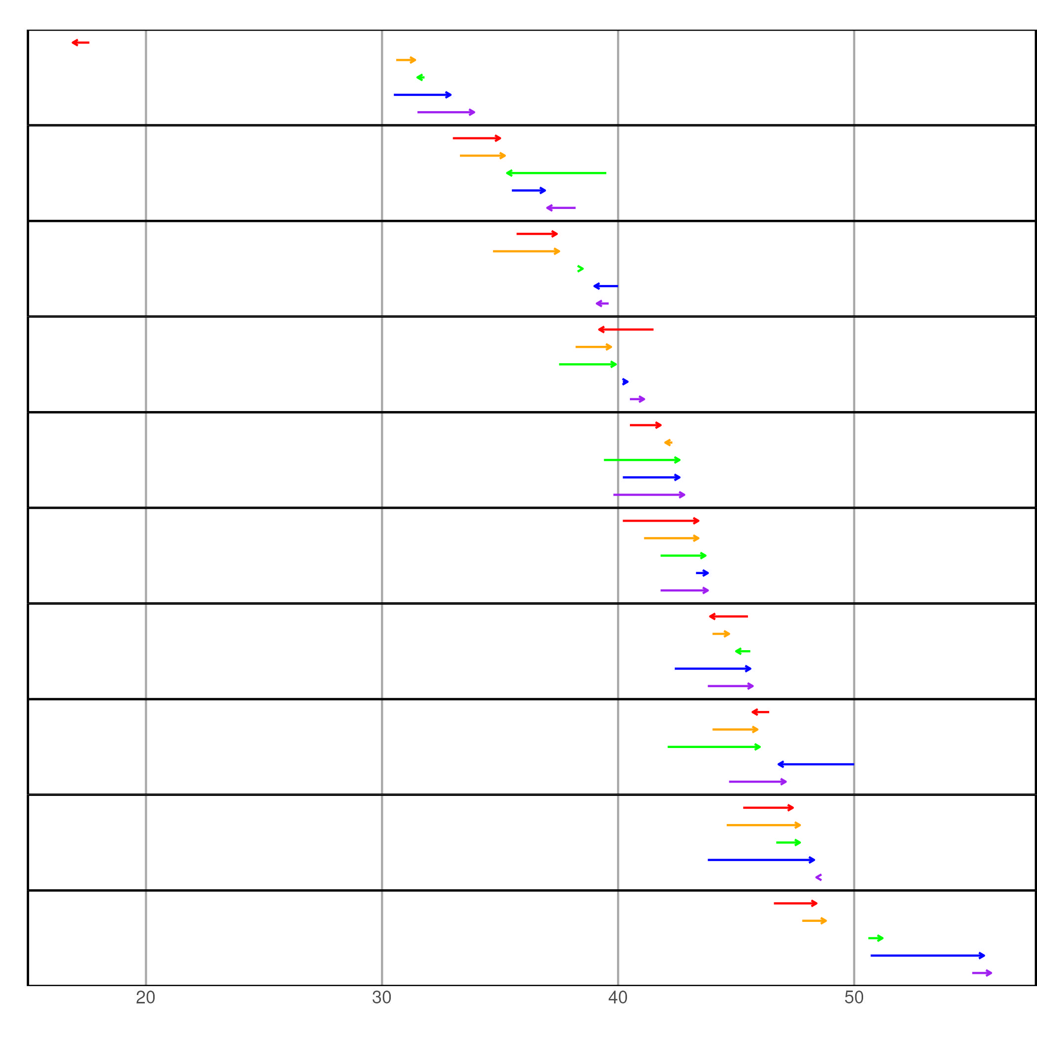
Our graph in Figure 6 looks like it will probably fit right in with the rest of the linked micromap plot. Now, we just need to put our code in proper function form:
> arrow_plot_build <- function(myPanel, myNumber, myNewStats, myAtts){+ myColors <- myAtts$colors+ myColumns <- myAtts[[myNumber]]$panel.data+ myNewStats$data1 <- myNewStats[, myColumns[1]]+ myNewStats$data2 <- myNewStats[, myColumns[2]]+ myPanel <- ggplot(myNewStats) ++ geom_segment(aes(x=data1, y=-pGrpOrd,+ xend= data2, yend=-pGrpOrd,+ colour=factor(color)),+ arrow=arrow(length=unit(0.1,"cm"))) ++ facet_grid(pGrp~.) ++ scale_colour_manual(values=myColors, guide="none")+ myPanel <- assimilatePlot(myPanel, myNumber, myAtts)+ }> myPanel
Dealing with a median row:
An additional issue to deal with is dealing with inserting a median row. There is a built in function that should handle this fairly we called alterForMedian. If, after we’ve added our new columns, we simply hand that function our stats table and the attributes list, it should give us back one that has been altered as needed. We also need to slightly alter the facet_grid line to allow for the median to be a different size.
> arrow_plot_build <- function(myPanel, myNumber, myNewStats, myAtts){+ myColors <- myAtts$colors+ myColumns <- myAtts[[myNumber]]$panel.data+ myNewStats$data1 <- myNewStats[, myColumns[1]]+ myNewStats$data2 <- myNewStats[, myColumns[2]]+ myNewStats <- alterForMedian(myNewStats, myAtts)+ myPanel <- ggplot(myNewStats) ++ geom_segment(aes(x=data1, y=-pGrpOrd,+ xend= data2, yend=-pGrpOrd,+ colour=factor(color)),+ arrow=arrow(length=unit(0.1,"cm"))) ++ facet_grid(pGrp~., space="free", scales="free_y") ++ scale_colour_manual(values=myColors, guide="none")+ myPanel <- assimilatePlot(myPanel, myNumber, myAtts)+ }> myPanel
After we run this function, or saving it to a file and then sourcing that file, we’ll be able to tell the mmplot function to build this graph simply entering a panel type of "arrow.plot".
Optional Step 4 - specializing user controlled attributes: If we run the line of code:
> print(myAtts)
We can see a full list of attributes available for alteration/specification by a user. All of these attributes (e.g. axis labels, background color, grid lines, etc.) are applied to the graph through the assimilatePlot function so if we like how our graph looks and don’t feel the need to give the user any more control on its features we can stop here. However, there might be some changes that users would like to make such as the width of the arrows and lengths of the arrow heads. In order to allow these changes by users we need to: a) create extra slots in our panel level of the attributes list and b) alter our code to recognize these options.
Creating the extra slots in the attribute list is actually not a terribly difficult process. This is done for every graph that has already been built into the micromap package. What these built in graphs have that ours is still lacking is a personalized "attribute function". When the mmplot function sees a panel type of "arrow.plot", it’s already looking for an attribute function called arrow.plot.att to supply the panel level list for our all encompassing attribute list that is being passed around, but we haven’t created this yet; so it settles on a built in function called standard.att. We’ll use standard.att to build our new arrow.plot.att function.
In the code below we first start with standard.att to get our useful base list, and then we append on the new attributes we’d like to control. We’ll call these new attributes "line.width" and "tip.length".
> myPanelAtts <- standard_att()> myPanelAtts <- append(myPanelAtts,+ list(line.width=1, tip.length=1))
Note that the "=1" is setting our defaults for these 2 entries at "1". We can control what "1" actually implies later. Now let’s put this into function form. Note that the mmplot function "sends" nothing to this function. It only wants a list of attributes back. Which makes our function simply look like:
> arrow_plot_att <- function(){+ myPanelAtts <- standard_att()+ myPanelAtts <- append(myPanelAtts,+ list(line.width=1, tip.length=1))+ }
Simple enough. Now let’s revisit our arrow.plot function and insert lines to pull these attribute specifications out of the attribute list and implement them in our graphing code:
> arrow_plot_build <- function(myPanel, myNumber, myNewStats, myAtts){+ myColors <- myAtts$colors+ myColumns <- myAtts[[myNumber]]$panel.data+ myLineWidth <- myAtts[[myNumber]]$line.width+ # Again, note that these are stored in the panel level section of the+ myTipLength <- myAtts[[myNumber]]$tip.length # attributes object+ myNewStats$data1 <- myNewStats[, myColumns[1]]+ myNewStats$data2 <- myNewStats[, myColumns[2]]+ myNewStats <- alterForMedian(myNewStats, myAtts)+ myPanel <- ggplot(myNewStats) ++ geom_segment(aes(x=data1, y=-pGrpOrd,+ xend= data2, yend=-pGrpOrd,+ colour=factor(color)),+ arrow=arrow(length=unit(0.1*myTipLength,"cm")),+ linewidth=myLineWidth) ++ facet_grid(pGrp~., space="free", scales="free_y") ++ scale_colour_manual(values=myColors, guide="none")+ myPanel <- assimilatePlot(myPanel, myNumber, myAtts)+ }> myPanel
Step Last: Now let’s try to implement this new panel in a simple linked micromap (using the statePolys map data from the initial example) and adjust the line width and tip length while we’re at it.
> mmplot(stat.data=myStats,+ map.data=statePolys,+ panel.types=c("map","labels", "arrow_plot"),+ panel.data=list(NA,"State", list("Rate_95","Rate_00")),+ ord.by="Rate_00",+ grouping=5,+ map.link=c("StateAb","ID"),+ panel.att=list(list(3, line.width=1.25, tip.length=1.5)),+ print.file="fig7.jpeg", print.res=100)
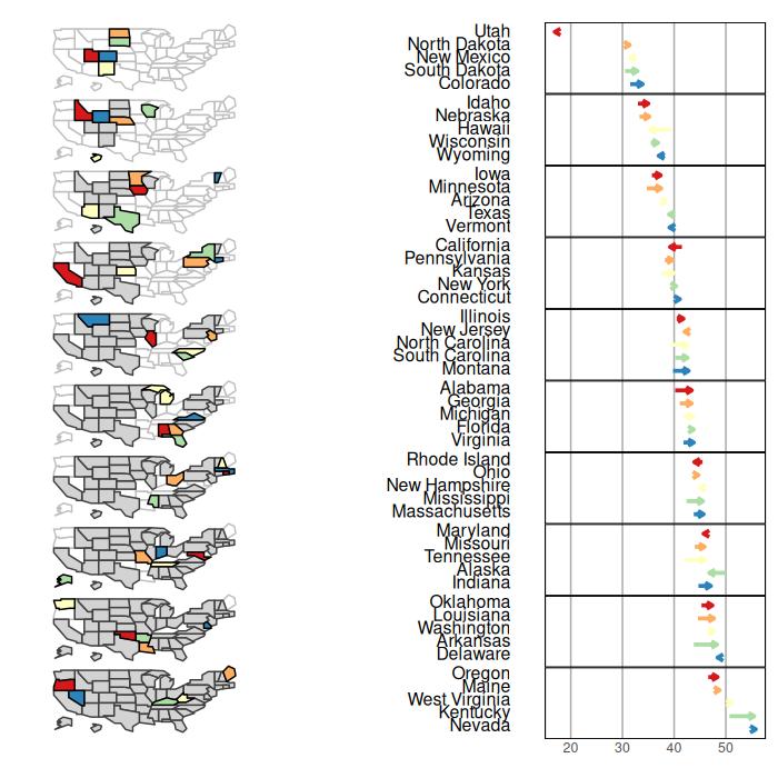
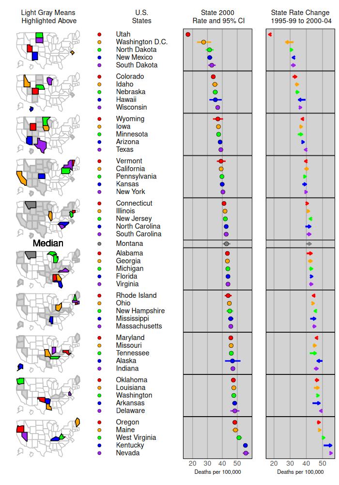
It looks like our new graph has been implemented nicely. We can obviously still clean this up a bit and might as well add in some extra plots as well. Also, we should bring Washington DC back into the picture (i.e. use our original myStats table) and make sure our median row is displaying correctly with the new graph. Using dot_legend we will add a legend and tweek the panel attributes section quite a bit, we are ready to present the following:
> data(lungMort)> myStats <- lungMort> mmplot(stat.data=myStats,+ map.data=statePolys,+ panel.types=c("map", "dot_legend", "labels", "dot_cl", "arrow_plot"),+ panel.data=list(NA,+ "points",+ "State",+ list("Rate_00","Lower_00","Upper_00"),+ list("Rate_95","Rate_00")),+ ord.by="Rate_00", grouping=5,+ median.row=T,+ map.link=c("StateAb","ID"),+ plot.height=10,+ colors=c("red","orange","green","blue","purple"),+ panel.att=list(list(1, header="Light Gray Means\n Highlighted Above",+ map.all=TRUE,+ fill.regions="two ended",+ inactive.fill="lightgray",+ inactive.border.color=gray(.7),+ inactive.border.size=2,+ panel.width=1),+ list(2, point.type=20,+ point.border=TRUE),+ list(3, header="U.S. \nStates ",+ panel.width=.8,+ align="left", text.size=.9),+ list(4, header="State 2000\n Rate and 95% CI",+ graph.bgcolor="lightgray",+ xaxis.ticks=list(20,30,40,50),+ xaxis.labels=list(20,30,40,50),+ xaxis.title="Deaths per 100,000"),+ list(5, header="State Rate Change\n 1995-99 to 2000-04",+ line.width=1.25, tip.length=1.5,+ graph.bgcolor="lightgray",+ xaxis.ticks=list(20,30,40,50),+ xaxis.labels=list(20,30,40,50),+ xaxis.title="Deaths per 100,000")),+ print.file="fig8.jpeg", print.res=100)
6 Group-Categorized Micromaps (mmgroupedplot function)
mmgroupedplot(stat.data, map.data, panel.types, panel.data, cat, map.link, …) The mmgroupedplot function is very similar to the mmplot function described earlier. With the mmplot function, we had a one-to-one relationship with one polygon being associated with one statistical summary that appeared as a single row in a perceptual group. With a group-categorized micromap, we are going to have a one-to-many relationship with one polygon now being associated with several statistical summaries. This one to many relationship is reflected in the structure of the statistical data table.
> library(micromap)> data("vegCov")> head(vegCov, n = 9)
Type Subpopulation Indicator1140 National National CondClassWgt4b.VEGCVR_COND1141 National National CondClassWgt4b.VEGCVR_COND1142 National National CondClassWgt4b.VEGCVR_COND1188 ecowsa3 EHIGH CondClassWgt4b.VEGCVR_COND1189 ecowsa3 EHIGH CondClassWgt4b.VEGCVR_COND1190 ecowsa3 EHIGH CondClassWgt4b.VEGCVR_COND1193 ecowsa3 PLNLOW CondClassWgt4b.VEGCVR_COND1194 ecowsa3 PLNLOW CondClassWgt4b.VEGCVR_COND1195 ecowsa3 PLNLOW CondClassWgt4b.VEGCVR_COND Category NResp Estimate.P StdError.P1140 1:LEAST DISTURBED 698 47.61908 1.5116431141 2:INTERMEDIATE DISTURBANCE 394 28.31880 1.5332171142 3:MOST DISTURBED 291 19.33501 1.2297591188 1:LEAST DISTURBED 129 42.16749 2.5970531189 2:INTERMEDIATE DISTURBANCE 92 30.70827 2.6859391190 3:MOST DISTURBED 48 17.58212 1.9904641193 1:LEAST DISTURBED 155 47.53334 2.7532671194 2:INTERMEDIATE DISTURBANCE 111 24.45491 2.5441081195 3:MOST DISTURBED 145 25.95537 2.341336 LCB95Pct.P UCB95Pct.P Estimate.U StdError.U LCB95Pct.U1140 44.65632 50.58185 516806.99 18907.163 479749.631141 25.31375 31.32385 307342.20 17184.380 273661.431142 16.92473 21.74529 209841.67 13516.940 183348.961188 37.07736 47.25762 187505.36 13383.579 161274.031189 25.44393 35.97261 136549.87 12402.806 112240.821190 13.68088 21.48336 78182.07 8887.312 60763.261193 42.13704 52.92965 186008.37 11785.392 162909.421194 19.46855 29.44127 95697.40 10313.978 75482.371195 21.36644 30.54430 101569.04 9522.937 82904.42 UCB95Pct.U1140 553864.351141 341022.961142 236334.391188 213736.691189 160858.931190 95600.881193 209107.311194 115912.421195 120233.65The polygons, or areas, that we want to use are listed under Subpopulation as “National”, “EHIGH”, “PLNLOW”, and “WMTNS”, and each of those areas are repeated three times in the statistical data to correspond to the three levels of disturbance listed under the Category column. We want to produce a micromap that has a panel showing the Estimate.P values crossed with the disturbance categories for each area. We want a similar panel produced using the Estimate.U values. We need to examine the spatial polgyon dataframe to see how it is structured. We will use the WSA3 spatial polygon data frame that has already been thinned.
> data("WSA3")> print(WSA3@data)
WSA_3 WSA_3_NM area_mdm ID1 EHIGH Eastern Highlands 1.197706e+12 EHIGH2 PLNLOW Plains and Lowlands 3.949916e+12 PLNLOW3 WMTNS West 2.640471e+12 WMTNS area_mdm area_mdm1 1.197676e+12 1.196321e+122 3.949854e+12 3.951018e+123 2.640467e+12 2.641354e+12Note that the column WSA_3 is potentially a good ID variable that could link the spatial and statistical data together. However, the WSA_3 column does not list “National”, but we can create that area after we make an inital map table using the create_map_table function.
> wsa.polys<-create_map_table(WSA3)> head(wsa.polys)
ID region poly coordsx coordsy hole plotorder plug1 EHIGH 1 2 672579.2 49281.8017 0 3 02 EHIGH 1 2 692236.2 27743.7400 0 3 03 EHIGH 1 2 662403.9 17823.7596 0 3 04 EHIGH 1 2 656638.2 3781.2090 0 3 05 EHIGH 1 2 643629.7 9115.8818 0 3 06 EHIGH 1 2 632432.9 -139.7886 0 3 0To create a National area, we can just use the perimeter outline from EHIGH, PLNLOW, and WMTNS and avoid using any of the interior polygons by setting “plug” and “hole” arguments to zero. Each of the polygons needs to have an unique number. Here is the code to create a National area and to assign a unique number to every polygon.
> national.polys<-subset(wsa.polys, hole==0 & plug==0)> national.polys<-transform(national.polys, ID="National", region=4,+ poly=region*1000 + poly)> head(national.polys)
ID region poly coordsx coordsy hole plotorder1 National 4 1002 672579.2 49281.8017 0 32 National 4 1002 692236.2 27743.7400 0 33 National 4 1002 662403.9 17823.7596 0 34 National 4 1002 656638.2 3781.2090 0 35 National 4 1002 643629.7 9115.8818 0 36 National 4 1002 632432.9 -139.7886 0 3 plug1 02 03 04 05 06 0
> wsa.polys<-rbind(wsa.polys,national.polys)> head(wsa.polys)
ID region poly coordsx coordsy hole plotorder plug1 EHIGH 1 2 672579.2 49281.8017 0 3 02 EHIGH 1 2 692236.2 27743.7400 0 3 03 EHIGH 1 2 662403.9 17823.7596 0 3 04 EHIGH 1 2 656638.2 3781.2090 0 3 05 EHIGH 1 2 643629.7 9115.8818 0 3 06 EHIGH 1 2 632432.9 -139.7886 0 3 0
> str(wsa.polys)
'data.frame':4626 obs. of 8 variables: $ ID : Factor w/ 4 levels "EHIGH","PLNLOW",..: 1 1 1 1 1 1 1 1 1 1 ... $ region : num 1 1 1 1 1 1 1 1 1 1 ... $ poly : num 2 2 2 2 2 2 2 2 2 2 ... $ coordsx : num 672579 692236 662404 656638 643630 ... $ coordsy : num 49282 27744 17824 3781 9116 ... $ hole : num 0 0 0 0 0 0 0 0 0 0 ... $ plotorder: num 3 3 3 3 3 3 3 3 3 3 ... $ plug : num 0 0 0 0 0 0 0 0 0 0 ...We assigned the National region equal to 4 as the other areas had already been assigned the values 1, 2, and 3 when we applied the create_map_table function. Note how the ID column in the map table can be linked to the Subpopulation column in the data table.
We can now produce the basic group-categorized micromap using syntax very similar to mmplot function. We now specify two new arguments “grp.by” and “cat”. The “grp”.by specifies the areas or polygons we are using from the statistical data, and “cat” specifies the categories that will be crossed with each of the areas.
> mmgroupedplot(stat.data=vegCov,+ map.data=wsa.polys,+ panel.types=c("map", "labels", "bar_cl", "bar_cl"),+ panel.data=list(NA,"Category",+ list("Estimate.P","LCB95Pct.P","UCB95Pct.P"),+ list("Estimate.U","LCB95Pct.U","UCB95Pct.U")),+ panel.att=list(list(2, panel.width = 1.5)),+ grp.by="Subpopulation",+ cat="Category",+ map.link=c("Subpopulation", "ID"),+ plot.width = 9,+ print.file="fig9.jpeg",print.res=100)
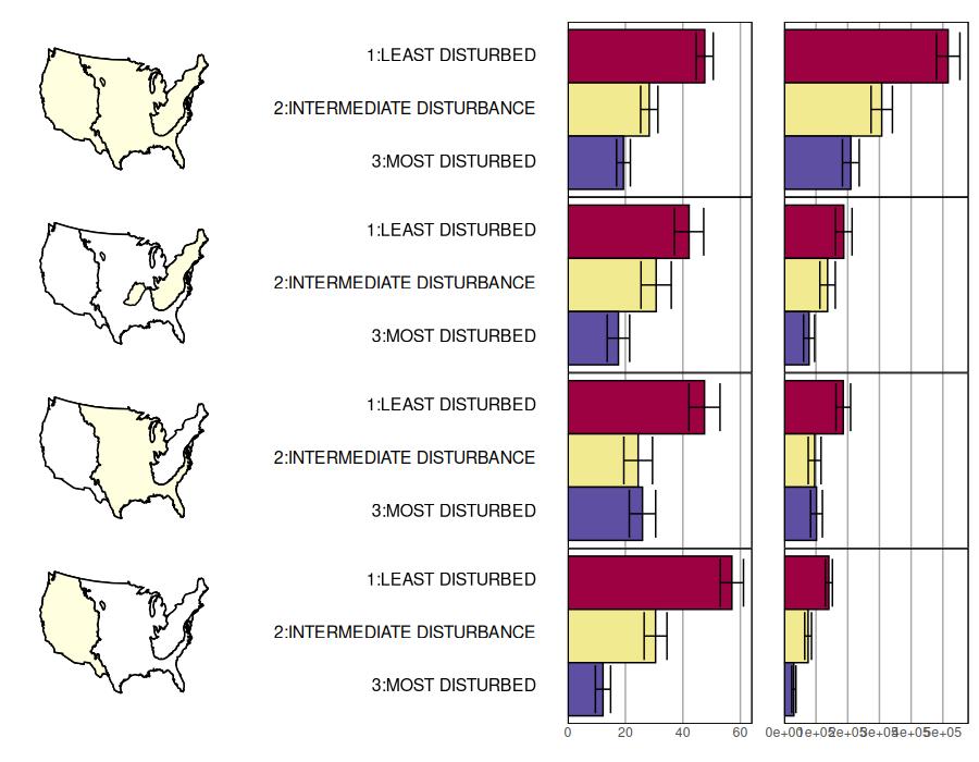
We can the refine that code to produce the finished version of a group-categorized micromap.
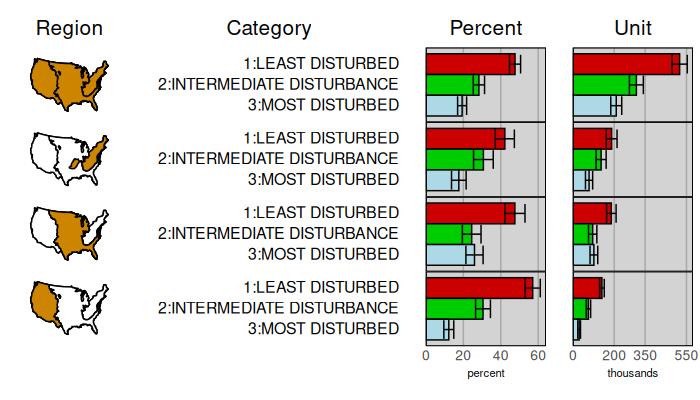
> mmgroupedplot(stat.data= vegCov,+ map.data= wsa.polys,+ panel.types=c("map", "labels", "bar_cl", "bar_cl"),+ panel.data=list(NA,"Category",+ list("Estimate.P","LCB95Pct.P","UCB95Pct.P"),+ list("Estimate.U","LCB95Pct.U","UCB95Pct.U")),+ grp.by="Subpopulation",+ cat="Category",+ colors=c("red3","green3","lightblue"),+ map.link=c("Subpopulation", "ID"),+ map.color="orange3",+ plot.grp.spacing=2,+ plot.width=7,+ plot.height=4,+ panel.att=list(list(1, header="Region", header.size=1.5,+ panel.width=.75),+ list(2, header="Category",+ header.size=1.5,+ panel.width=2),+ list(3, header="Percent", header.size=1.5,+ graph.bgcolor="lightgray",+ xaxis.title="percent",+ xaxis.ticks=list(0,20,40,60),+ xaxis.labels=list(0,20,40,60)),+ list(4, header="Unit", header.size=1.5,+ graph.bgcolor="lightgray",+ xaxis.title="thousands",+ xaxis.ticks=list(0,200000,350000,550000),+ xaxis.labels=list(0,200,350,550))),+ print.file="fig10.jpeg",print.res=100)
7 Using the sf package with micromap
The micromap package primarily uses the sp package to work with spatially referenced data. This approach was created with the assumption that micromap users must first combine their data with spatial polygons using the create_map_table function, i.e., data are often collected separately prior to linking with any spatial attributes. The sf (simple features) package is a newer and more popular approach in R for working with spatial data that combines both attribute and geometry (spatial) data in a single object. Using data in the simple features format with micromap may be preferred by users familiar with the package. The approach may also be preferred if the attribute and spatial data are already together, e.g., in a shapefile with attributes.
Using sf spatial objects with micromap follows a similar workflow as with sp objects, with the exception that the feature data does not need to be explicitly linked to the spatial data before plotting. In other words, the create_map_table function does not need to be used before plotting. The stat.data and map.link arguments in mmplot are also not required for a sf object.
Below shows a simple example using micromap with a sf spatial object. The nc dataset from the sf package is first loaded from disk.
> library(sf)> nc <- st_read(system.file("shape/nc.shp", package="sf"), quiet=T)> head(nc)
Simple feature collection with 6 features and 14 fieldsGeometry type: MULTIPOLYGONDimension: XYBounding box: xmin: -81.74107 ymin: 36.07282 xmax: -75.77316 ymax: 36.58965Geodetic CRS: NAD27 AREA PERIMETER CNTY_ CNTY_ID NAME FIPS FIPSNO1 0.114 1.442 1825 1825 Ashe 37009 370092 0.061 1.231 1827 1827 Alleghany 37005 370053 0.143 1.630 1828 1828 Surry 37171 371714 0.070 2.968 1831 1831 Currituck 37053 370535 0.153 2.206 1832 1832 Northampton 37131 371316 0.097 1.670 1833 1833 Hertford 37091 37091 CRESS_ID BIR74 SID74 NWBIR74 BIR79 SID79 NWBIR791 5 1091 1 10 1364 0 192 3 487 0 10 542 3 123 86 3188 5 208 3616 6 2604 27 508 1 123 830 2 1455 66 1421 9 1066 1606 3 11976 46 1452 7 954 1838 5 1237 geometry1 MULTIPOLYGON (((-81.47276 3...2 MULTIPOLYGON (((-81.23989 3...3 MULTIPOLYGON (((-80.45634 3...4 MULTIPOLYGON (((-76.00897 3...5 MULTIPOLYGON (((-77.21767 3...6 MULTIPOLYGON (((-76.74506 3...
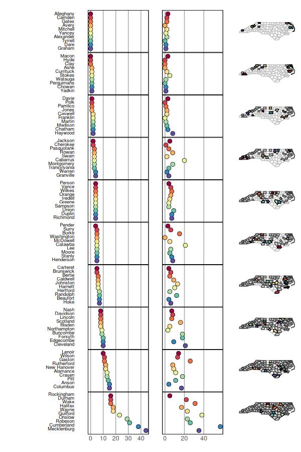
The mmplot function is then used, where the primary difference is that the stat.data and map.link arguments are not needed for a sf object. Instead, the complete nc data object is passed to the map.data argument. All other arguments are used as before.
> mmplot(map.data=nc,+ panel.types=c("labels", "dot","dot", "map"),+ panel.data=list("NAME","SID74","SID79", NA),+ ord.by="SID74", grouping=10,+ median.row=F,+ print.file="fig11.jpeg",+ print.res=100,+ plot.height=9,+ plot.width=6,+ panel.att=list(list(1, text.size=0.6))+ )