How to use the psych package for regression and mediation analysis
1 Overview of this and related documents
To do basic and advanced personality and psychological research using R is not as complicated as some think. This is one of a set of “How To” to do various things using R (R Core Team, 2023), particularly using the psych (Revelle, 2025) package.
The current list of How To’s includes:
- 1.
An introduction (vignette) of the psych package
- 2.
An overview (vignette) of the psych package
- 3.
Installing R and some useful packages
- 4.
- 5.
Using R and the psych for factor analysis and principal components analysis.
- 6.
Using the scoreItems function to find scale scores and scale statistics.
- 7.
Using mediate and lmCor to do mediation, moderation and regression analysis (this document)
1.1 Jump starting the psych package–a guide for the impatient
You have installed psych and you want to use it without reading much more. What should you do?
- 1.
Activate the psych and psychTools packages.
> library(psych)> library(psychTools)
- 2.
Input your data. If your file name ends in .sav, .text, .txt, .csv, .xpt, .rds, .Rds, .rda, or .RDATA, then just read it in directly using read.file. Or you can go to your friendly text editor or data manipulation program (e.g., Excel) and copy the data to the clipboard. Include a first line that has the variable labels. Paste it into psych using the read.clipboard.tab command:
myData <- read.file() #this will open a search window on your machine# and read or load the file.#or#first copy your file to your clipboard and thenmyData <- read.clipboard.tab() #if you have an excel file
- 3.
Make sure that what you just read is right. Describe it and perhaps look at the first and last few lines. If you want to “view" the first and last few lines using a spreadsheet like viewer, use quickView.
describe(myData)headTail(myData)#orquickView(myData)
- 4.
Look at the patterns in the data. If you have fewer than about 10 variables, look at the SPLOM (Scatter Plot Matrix) of the data using pairs.panels.
pairs.panels(myData)
- 5.
Find the correlations of all of your data.
- •
Descriptively (just the values)
lowerCor(myData)
- •
Graphically
corPlot(myData) #show the numbers, #scales the character size by "significance"corPlot(myData,scale=FALSE) #show the numbers, # all characters the same sizecorPlot(lowerCor(myData), numbers =TRUE) #print the correlations # and show them graphically
- •
1.2 For the not impatient
The following pages are meant to lead you through the use of the lmCor and mediate functions. The assumption is that you have already made psych active and want some example code.
2 Multiple regression and mediation
Mediation and moderation are merely different uses of the linear model and are implemented in psych with two functions: lmCor and mediate.
Given a set of predictor variables, and a set of criteria variables, , multiple regression solves the equation by finding where is the covariances of the variables and is the covariances of predictors and the criteria.
Although typically done using the raw data, clearly this can also be done by using the covariance or correlation matrices. lmCor was developed to handle the correlation matrix solution but has been generalized to the case of raw data. In the later case, it assumes a Missing Completely at Random (MCAR) structure, and thus uses all the data and finds pair.wise complete correlations. For complete data sets, the results are identical to using lm. By default, lmCor uses standardized variables, but to compare with lm, it can use unstandardized variables.
3 Regression using lmCor
Although typically done from a raw data matrix (using the lm function), it is sometimes useful to do the regression from a correlation or covariance matrix. lmCor was developed for this purpose. From a correlation/covariance matrix, it will do normal regression as well as regression on partialled correlation matrices. With the raw data, it will also do moderated regression (centered or non-centered). In particular, for the raw data, it will work with missing data.
An interesting option, if using categorical or dichotomous data is first find the appropriate polychoric, tetrachoric, or poly-serial correlations using mixedCor and then use the resulting correlation matrix for analysis. The resulting correlations and multiple correlations will not match those of the lm analysis.
3.1 Comparison with lm on complete data
Use the attitude data set for our first example.
3.1.1 It is important to know your data by describing it first
> psych::describe(attitude)
vars n mean sd median trimmed mad min max range skewrating 1 30 64.63 12.17 65.5 65.21 10.38 40 85 45 -0.36complaints 2 30 66.60 13.31 65.0 67.08 14.83 37 90 53 -0.22privileges 3 30 53.13 12.24 51.5 52.75 10.38 30 83 53 0.38learning 4 30 56.37 11.74 56.5 56.58 14.83 34 75 41 -0.05raises 5 30 64.63 10.40 63.5 64.50 11.12 43 88 45 0.20critical 6 30 74.77 9.89 77.5 75.83 7.41 49 92 43 -0.87advance 7 30 42.93 10.29 41.0 41.83 8.90 25 72 47 0.85 kurtosis serating -0.77 2.22complaints -0.68 2.43privileges -0.41 2.23learning -1.22 2.14raises -0.60 1.90critical 0.17 1.81advance 0.47 1.88
3.1.2 Now do the regressions
> #do not standardize> mod1 <- lmCor(rating ~ complaints + privileges, data=attitude,std=FALSE)> mod1
Call: lmCor(y = rating ~ complaints + privileges, data = attitude, std = FALSE)Multiple Regression from raw data DV = rating slope se t p lower.ci upper.ci VIF Vy.x r(Intercept) 15.33 7.16 2.14 4.1e-02 0.64 30.02 1.00 0.00 0.00complaints 0.78 0.12 6.54 5.2e-07 0.54 1.03 1.45 0.70 133.78privileges -0.05 0.13 -0.39 7.0e-01 -0.32 0.22 1.45 -0.02 63.46Residual Standard Error = 7.1 with 27 degrees of freedom Multiple Regression R R2 Ruw R2uw Shrunken R2 SE of R2 overall F df1 df2 prating 0.83 0.68 0.71 0.5 0.66 0.08 29.1 2 27 1.83e-07
Compare this solution with the results of the lm function.
> summary(lm(rating ~ complaints + privileges, data=attitude))
Call:lm(formula = rating ~ complaints + privileges, data = attitude)Residuals: Min 1Q Median 3Q Max-12.7887 -5.6893 -0.0284 6.2745 9.9726Coefficients: Estimate Std. Error t value Pr(>|t|)(Intercept) 15.32762 7.16023 2.141 0.0415 *complaints 0.78034 0.11939 6.536 5.22e-07 ***privileges -0.05016 0.12992 -0.386 0.7025---Signif. codes: 0 ‘***’ 0.001 ‘**’ 0.01 ‘*’ 0.05 ‘.’ 0.1 ‘ ’ 1Residual standard error: 7.102 on 27 degrees of freedomMultiple R-squared: 0.6831,Adjusted R-squared: 0.6596F-statistic: 29.1 on 2 and 27 DF, p-value: 1.833e-07
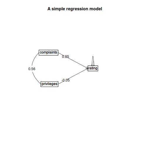
The graphic for the standardized regression is shown in (Figure 1).
Call: lmCor(y = rating ~ complaints + privileges, data = attitude)Multiple Regression from raw data DV = rating slope se t p lower.ci upper.ci VIF Vy.x r(Intercept) 0.00 0.11 0.00 1.0e+00 -0.22 0.22 1.00 0.00 0.00complaints 0.85 0.13 6.54 5.2e-07 0.59 1.12 1.45 0.70 0.83privileges -0.05 0.13 -0.39 7.0e-01 -0.32 0.22 1.45 -0.02 0.43Residual Standard Error = 0.58 with 27 degrees of freedom Multiple Regression R R2 Ruw R2uw Shrunken R2 SE of R2 overall F df1 df2 prating 0.83 0.68 0.71 0.5 0.66 0.08 29.1 2 27 1.83e-07
pdf 2
3.2 From a correlation matrix
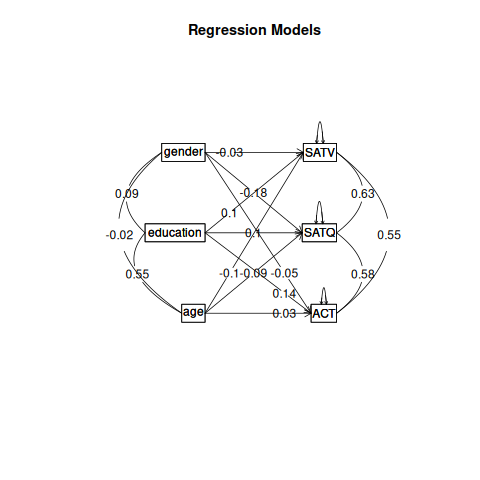
Perhaps most usefully, lmCor will find the beta weights between a set of X variables, and a set of Y variables. Consider seven variables in the atttitude data set. We first find the correlation matrix (normally, this could just be supplied by the user). Then we find the regressions from the correlation matrix. Compare this regression to the (standardized) solution shown above. By specifying the number of observations (n.obs), we are able to apply various inferential tests.
> R <- lowerCor(attitude)
ratng cmpln prvlg lrnng raiss crtcl advncrating 1.00complaints 0.83 1.00privileges 0.43 0.56 1.00learning 0.62 0.60 0.49 1.00raises 0.59 0.67 0.45 0.64 1.00critical 0.16 0.19 0.15 0.12 0.38 1.00advance 0.16 0.22 0.34 0.53 0.57 0.28 1.00
> lmCor(rating ~ complaints + privileges, data=R, n.obs =30)
Call: lmCor(y = rating ~ complaints + privileges, data = R, n.obs = 30)Multiple Regression from matrix input DV = rating slope se t p lower.ci upper.ci VIF Vy.x rcomplaints 0.85 0.13 6.54 5.2e-07 0.59 1.12 1.45 0.70 0.83privileges -0.05 0.13 -0.39 7.0e-01 -0.32 0.22 1.45 -0.02 0.43Residual Standard Error = 0.58 with 27 degrees of freedom Multiple Regression R R2 Ruw R2uw Shrunken R2 SE of R2 overall F df1 df2 prating 0.83 0.68 0.71 0.5 0.66 0.08 29.1 2 27 1.83e-07
Compare this solution (from the correlation matrix) with the standardized solution for the raw data. lmCor does several things:
- •
Finds the regression weights (betas) between the predictor variables and each of the criterion variables.
- •
If the number of subjects is specified, or if the raw data are used, it also compares each of these betas to its standard error, finds a statistic, and reports the probability of the .
- •
It reports the Multiple R and based upon these beta weights. In addition, following the tradition of the robust beauty of the improper linear models (Dawes, 1979) it also reports the unit weighted multiple correlations.
- •
If there are more than 1 Y variables, the canonical correlations between the two sets (X and Y) (Hotelling, 1936) arereported. The canonical loadings are reported in the Xmat and Ymat objects.
- •
Cohen’s set correlation (Cohen, 1982) as well as the unweighted correlation between the two sets of variables are reported.
3.3 The Hotelling example
> #the second Kelley data from Hotelling> kelley <- structure(list(speed = c(1, 0.4248, 0.042, 0.0215, 0.0573), power = c(0.4248,+ 1, 0.1487, 0.2489, 0.2843), words = c(0.042, 0.1487, 1, 0.6693,+ 0.4662), symbols = c(0.0215, 0.2489, 0.6693, 1, 0.6915), meaningless = c(0.0573,+ 0.2843, 0.4662, 0.6915, 1)), .Names = c("speed", "power", "words",+ "symbols", "meaningless"), class = "data.frame", row.names = c("speed",+ "power", "words", "symbols", "meaningless"))> #first show the correlations> lowerMat(kelley)
speed power words symbl mnnglspeed 1.00power 0.42 1.00words 0.04 0.15 1.00symbols 0.02 0.25 0.67 1.00meaningless 0.06 0.28 0.47 0.69 1.00
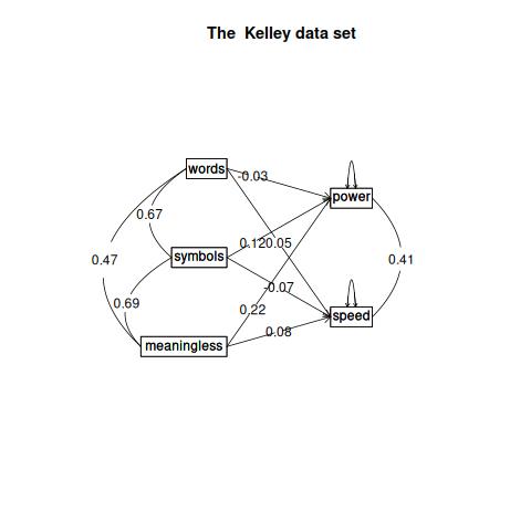
> #now find and draw the regression> sc <- lmCor(power + speed ~ words + symbols + meaningless,data=kelley) #formula mode> sc #show it
Call: lmCor(y = power + speed ~ words + symbols + meaningless, data = kelley)Multiple Regression from matrix input DV = power slope VIF Vy.x rwords -0.03 1.81 -0.01 0.15symbols 0.12 2.72 0.03 0.25meaningless 0.22 1.92 0.06 0.28 Multiple Regression R R2 Ruw R2uwpower 0.29 0.09 0.26 0.07 DV = speed slope VIF Vy.x rwords 0.05 1.81 0 0.04symbols -0.07 2.72 0 0.02meaningless 0.08 1.92 0 0.06 Multiple Regression R R2 Ruw R2uwspeed 0.07 0.01 0.05 0Various estimates of between set correlationsSquared Canonical Correlations[1] 0.1036 0.0032 Average squared canonical correlation = 0.05 Cohen's Set Correlation R2 = 0.1Unweighted correlation between the two sets = 0.18
A plot of the regression model is shown as well (Figure 2).
pdf 2
3.4 Canonical Correlation using lmCor
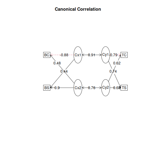
A generalization of multiple regression to multiple predictors and multiple criteria is canonical correlation (Hotelling, 1936). Given a partitioning of a correlation matrix, R, into Rxx, Ryy and Rxy, canonical correlation finds orthogonal components of the correlations between the Rx and Ry sets (the Rxy correlations). Consider the Kelley data set discussed by Hotelling (1936) who introduced the canonical correlation. This analysis is shown in help menu for lmCor. Another data set is the “Belly Dancer" data set discussed by Tabachnick and Fidell (2001) (Chapter 12). Here I show the data, the correlations, the regressions, and the canonical correlations.
> dancer <- structure(list(TS = c(1, 7, 4.6, 1, 7, 7, 7, 7), TC = c(1, 1,+ 5.6, 6.6, 4.9, 7, 1, 1), BS = c(1, 7, 7, 1, 7, 6.4, 7, 2.4),+ BC = c(1, 1, 7, 5.9, 2.9, 3.8, 1, 1)), class = "data.frame", row.names = c(NA,+ -8L))> dancer #show the data
TS TC BS BC1 1.0 1.0 1.0 1.02 7.0 1.0 7.0 1.03 4.6 5.6 7.0 7.04 1.0 6.6 1.0 5.95 7.0 4.9 7.0 2.96 7.0 7.0 6.4 3.87 7.0 1.0 7.0 1.08 7.0 1.0 2.4 1.0
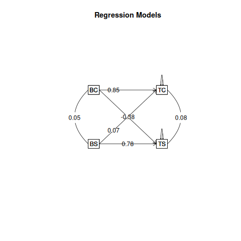
> model <- psych::lmCor(TC + TS ~ BC + BS, data = dancer)> summary(model) #show the summary statistics
Multiple Regression from raw datapsych::lmCor(y = TC + TS ~ BC + BS, data = dancer)Multiple Regression from matrix inputBeta weights and raw correlations TC TS TC TS(Intercept) 0.000 0.00 0.00 0.00BC 0.854 -0.38 0.86 -0.34BS 0.066 0.78 0.11 0.76Multiple R TC TS0.86 0.85Multiple R2 TC TS0.74 0.72Cohen's set correlation R2[1] 0.93Squared Canonical Correlations[1] 0.84 0.58
> round(model$Xmat,2) #the X canonical loadings
Cx1 Cx2BC -0.88 0.48BS 0.44 0.90
> round(model$Ymat,2) #the Y canonical loadings
Cy1 Cy2TC -0.79 0.62TS 0.74 0.68
> cancorDiagram(model, main="Canonical correlations for the 'Belly Dancer' example") #and the associated canonical figure>
> png('dancerlm.png')
> model <- psych::lmCor(TC + TS ~ BC + BS, data = dancer)
> dev.off()
2
> png('dancer.png')
> cancorDiagram(model)
> dev.off()
2
But, we can also do multiple predictors and multiple criteria in the same call:
pdf 2
3.5 Graphic displays
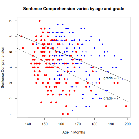
When considering the within group relationships for multiple groups, (e.g., gender or grade level) it is useful to draw separate regression lines for each group. Consider the case of the regression of age on paragraph comprehension as a function of class grade (6 or 7) in the holzinger.swineford data set in psychTools.
> lowerCor(holzinger.swineford[c(3,7,12:14)])
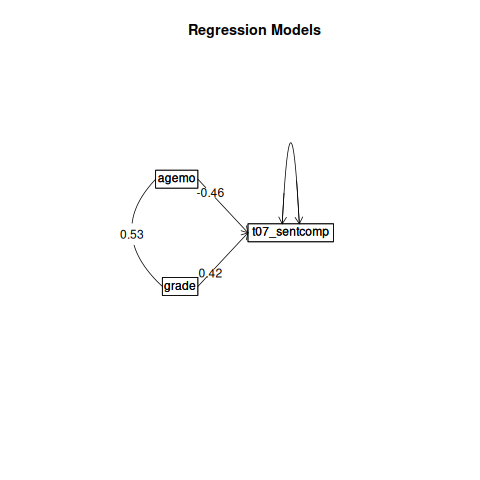
grade agemo t05_g t06_p t07_sgrade 1.00agemo 0.53 1.00t05_geninfo 0.21 -0.15 1.00t06_paracomp 0.21 -0.20 0.66 1.00t07_sentcomp 0.18 -0.23 0.72 0.73 1.00It would seem as if both age and grade account for 4% of the variance in paragraph comprehension. But combining these two in a multiple regression increases the variance explained from 8% (the sum of the two) to 18%, because age and grade suppress variance unrelated to cognitive performance.
Show this finding in two different ways: as a plot of the separate regression lines Figure 6 for each grade or as a simple path model Figure 7 . Note that because grade goes from 7 to 8, to index the colors in the plot we subtract 6 from both grades to get a 1, 2 variable.
> png('hs.png')> plot(t07_sentcomp ~ agemo, col=c("red","blue")[holzinger.swineford$grade -6],+ pch=26-holzinger.swineford$grade,data=holzinger.swineford,+ ylab="Sentence Comprehension",xlab="Age in Months",+ main="Sentence Comprehension varies by age and grade")> by(holzinger.swineford, holzinger.swineford$grade -6,function(x) abline(+ lmCor(t07_sentcomp ~ agemo,data=x, std=FALSE, plot=FALSE) ,lty=c("dashed","solid")[x$grade-6]))
holzinger.swineford$grade - 6: 1NULL------------------------------------------------------------holzinger.swineford$grade - 6: 2NULL
> text(190,3.3,"grade = 8")> text(190,2,"grade = 7")> dev.off()
pdf 2
> png('hsp.png')> lmCor(t07_sentcomp ~ agemo + grade,data=holzinger.swineford)
Call: lmCor(y = t07_sentcomp ~ agemo + grade, data = holzinger.swineford)Multiple Regression from raw data DV = t07_sentcomp slope se t p lower.ci upper.ci VIF Vy.x r(Intercept) 0.00 0.05 0.00 1.0e+00 -0.10 0.10 1.00 0.00 0.00agemo -0.46 0.06 -7.39 1.5e-12 -0.58 -0.34 1.39 0.11 -0.23grade 0.42 0.06 6.78 6.4e-11 0.30 0.54 1.39 0.07 0.18Residual Standard Error = 0.91 with 298 degrees of freedom Multiple Regression R R2 Ruw R2uw Shrunken R2 SE of R2 overall F df1 df2t07_sentcomp 0.43 0.18 -0.03 0 0.18 0.04 32.97 2 298 pt07_sentcomp 1.16e-13
> dev.off()
pdf 2
To show just the coefficients of this model, do the regressions without the plot, turn off the plot option:
> by(holzinger.swineford,holzinger.swineford$grade,function(x)+ lmCor(t07_sentcomp ~ agemo,data=x, std=FALSE, plot=FALSE) )
holzinger.swineford$grade: 7Call: lmCor(y = t07_sentcomp ~ agemo, data = x, std = FALSE, plot = FALSE)Multiple Regression from raw data DV = t07_sentcomp slope se t p lower.ci upper.ci VIF Vy.x r(Intercept) 12.10 1.37 8.83 2.1e-15 9.39 14.81 1 0.00 0.00agemo -0.05 0.01 -5.83 3.0e-08 -0.07 -0.03 1 0.18 -5.61Residual Standard Error = 1.15 with 155 degrees of freedom Multiple Regression R R2 Ruw R2uw Shrunken R2 SE of R2 overall F df1 df2t07_sentcomp 0.42 0.18 -0.42 0.18 0.17 0.05 34.04 1 155 pt07_sentcomp 3.05e-08------------------------------------------------------------holzinger.swineford$grade: 8Call: lmCor(y = t07_sentcomp ~ agemo, data = x, std = FALSE, plot = FALSE)Multiple Regression from raw data DV = t07_sentcomp slope se t p lower.ci upper.ci VIF Vy.x r(Intercept) 12.09 1.64 7.38 1.2e-11 8.85 15.33 1 0.00 0.00agemo -0.04 0.01 -4.59 9.5e-06 -0.06 -0.03 1 0.13 -4.74Residual Standard Error = 1.2 with 142 degrees of freedom Multiple Regression R R2 Ruw R2uw Shrunken R2 SE of R2 overall F df1 df2t07_sentcomp 0.36 0.13 -0.36 0.13 0.12 0.05 21.11 1 142 pt07_sentcomp 9.5e-06
3.6 Moderated multiple regression
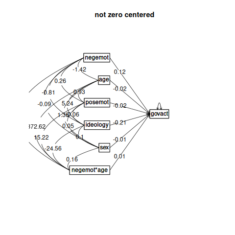
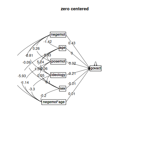
With the raw data, find interactions (known as moderated multiple regression). This is done by zero centering the data (Cohen et al., 2003) and then multiplying the two terms of the interaction. As an option, do not zero center the data (Hayes, 2013) which results in different “main effects" but the same interaction term. To show the equivalence of the interaction terms, we also must not standardize the results.
Use the globalWarm data set taken from (Hayes, 2013)
> mod <-lmCor(govact ~ negemot * age + posemot +ideology+sex,data=globalWarm,+ std=FALSE, zero=FALSE, plot=FALSE)> mod
Call: lmCor(y = govact ~ negemot * age + posemot + ideology + sex, data = globalWarm, std = FALSE, plot = FALSE, zero = FALSE)Multiple Regression from raw data DV = govact slope se t p lower.ci upper.ci VIF Vy.x r(Intercept) 5.17 0.34 15.29 1.6e-46 4.51 5.84 1.00 0.00 0.00negemot 0.12 0.08 1.45 1.5e-01 -0.04 0.28 11.59 0.08 1.20age -0.02 0.01 -3.99 7.1e-05 -0.04 -0.01 6.95 0.03 -2.16posemot -0.02 0.03 -0.77 4.4e-01 -0.08 0.03 1.03 0.00 0.08ideology -0.21 0.03 -7.88 1.0e-14 -0.26 -0.16 1.20 0.10 -0.86sex -0.01 0.08 -0.15 8.8e-01 -0.16 0.14 1.05 0.00 -0.07negemot*age 0.01 0.00 4.10 4.5e-05 0.00 0.01 16.46 0.20 57.75Residual Standard Error = 1.06 with 808 degrees of freedom Multiple Regression R R2 Ruw R2uw Shrunken R2 SE of R2 overall F df1 df2 pgovact 0.63 0.4 0.15 0.02 0.4 0.03 90.08 6 808 1.82e-86
> mod0 <- lmCor(govact ~ negemot * age + posemot +ideology+sex,data=globalWarm,std=FALSE, plot=FALSE)> mod0
Call: lmCor(y = govact ~ negemot * age + posemot + ideology + sex, data = globalWarm, std = FALSE, plot = FALSE)Multiple Regression from raw data DV = govact slope se t p lower.ci upper.ci VIF Vy.x r(Intercept) 4.60 0.04 123.92 0.0e+00 4.52 4.67 1.00 0.00 0.00negemot 0.43 0.03 16.51 5.8e-53 0.38 0.48 1.17 0.28 1.20age 0.00 0.00 -0.58 5.6e-01 -0.01 0.00 1.07 0.00 -2.16posemot -0.02 0.03 -0.77 4.4e-01 -0.08 0.03 1.03 0.00 0.08ideology -0.21 0.03 -7.88 1.0e-14 -0.26 -0.16 1.20 0.10 -0.86sex -0.01 0.08 -0.15 8.8e-01 -0.16 0.14 1.05 0.00 -0.07negemot*age 0.01 0.00 4.10 4.5e-05 0.00 0.01 1.01 0.02 5.92Residual Standard Error = 1.06 with 808 degrees of freedom Multiple Regression R R2 Ruw R2uw Shrunken R2 SE of R2 overall F df1 df2 pgovact 0.63 0.4 0.07 0.01 0.4 0.03 90.08 6 808 1.82e-86
pdf 2
pdf 2
3.7 Plotting the interactions
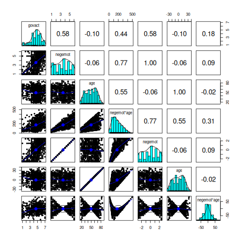
To visualize the effect of zero (mean) centering, it is useful to plot the various elements that go into the linear model. lmCor returns the product terms as well as the original data. Combine the two datasets to make it clearer. Note that the correlations of the centered age, negemot with the uncentered are 1.0, but that the correlations with the product terms depend upon centering versus not. Drop some of the other variables from the figure for clarity (Figure 10).
pdf 2
3.8 Comparisons to lm
The lmCor function duplicates the functionality of the lm function for complete data, although lm does not zero center and lmCor will (by default). In addition, lmCor finds correlations based upon pair.wise deletion of missing data, while lm does case.wise deletion. We compare the lm and lmCor results for complete data by setting the use = "complete" option. Use the sat.act data set which has some missing values.
> summary(lm(SATQ ~ SATV*gender + ACT, data=sat.act))
Call:lm(formula = SATQ ~ SATV * gender + ACT, data = sat.act)Residuals: Min 1Q Median 3Q Max-296.210 -45.738 4.323 52.355 252.306Coefficients: Estimate Std. Error t value Pr(>|t|)(Intercept) 138.52395 61.18770 2.264 0.0239 *SATV 0.50280 0.10030 5.013 6.84e-07 ***gender -22.24995 35.59228 -0.625 0.5321ACT 7.71702 0.77707 9.931 < 2e-16 ***SATV:gender -0.01984 0.05706 -0.348 0.7281---Signif. codes: 0 ‘***’ 0.001 ‘**’ 0.01 ‘*’ 0.05 ‘.’ 0.1 ‘ ’ 1Residual standard error: 81.18 on 682 degrees of freedom (13 observations deleted due to missingness)Multiple R-squared: 0.51,Adjusted R-squared: 0.5071F-statistic: 177.5 on 4 and 682 DF, p-value: < 2.2e-16
> mod <- lmCor(SATQ ~ SATV*gender + ACT, data=(sat.act), zero=FALSE, std=FALSE,use="complete")> print(mod,digits=5)
Call: lmCor(y = SATQ ~ SATV * gender + ACT, data = (sat.act), use = "complete", std = FALSE, zero = FALSE)Multiple Regression from raw data DV = SATQ slope se t p lower.ci upper.ci VIF(Intercept) 138.52395 61.18770 2.26392 2.3892e-02 18.38505 258.66284 1.00000SATV 0.50280 0.10030 5.01295 6.8399e-07 0.30587 0.69973 13.43994gender -22.24995 35.59228 -0.62513 5.3209e-01 -92.13355 47.63365 30.29663ACT 7.71702 0.77707 9.93090 8.4691e-22 6.19128 9.24276 1.46678SATV*gender -0.01984 0.05706 -0.34775 7.2814e-01 -0.13188 0.09219 41.25607 Vy.x r(Intercept) 0.00000 0.00000SATV 0.31739 8441.18530gender 0.01525 -9.16307ACT 0.18928 327.98982SATV*gender -0.01191 8027.53275Residual Standard Error = 81.18474 with 682 degrees of freedom Multiple Regression R R2 Ruw R2uw Shrunken R2 SE of R2 overall F df1 df2SATQ 0.71414 0.51 0.44175 0.19515 0.50712 0.02645 177.4575 4 682 pSATQ 3.98472e-104
4 Mediation using the mediate function
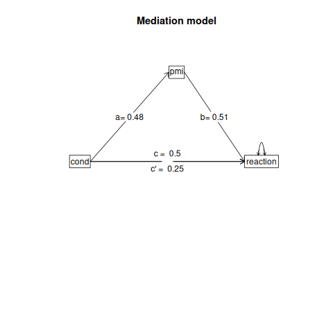
Mediation analysis is just linear regression reorganized slightly to show the direct effects of an X variable upon Y, partialling out the effect of a “mediator" (Figure 11). Although the statistical “significance" of the (c) path and the (c’) path are both available from standard regression, the mediation effect (ab) is best found by boot strapping the regression model and displaying the empirical confidence intervals.
A number of papers discuss how to test for the effect of mediation and there are some very popular ‘macros’ for SPSS and SAS to do so (Hayes, 2013; Preacher and Hayes, 2004; Preacher et al., 2007; Preacher, 2015). A useful discussion of mediation and moderation with sample data sets is found in Hayes (2013). More recently, the processR package (Moon, 2020) has been released with these data sets. Although these data used to be be available from Hayes’ website, that site seems to have vanished. I use these for comparisons with the results in Hayes (2013). Four of these data sets are now included in the psych package with the kind permission of their authors: Garcia is from Garcia et al. (2010), and Tal_Or is from Tal-Or et al. (2010), The Pollack correlation matrix is taken from an article by Pollack et al. (2012). The globalWarm data set is the glbwarm data set in the processR package and added to psychTools with the kind permission of the original author, Erik Nisbet.
To find the confidence intervals of the effect of mediation (the reduction between the c and c’ paths, where c’ = c - ab), bootstrap the results by randomly sampling from the data with replacement (e.g n.iter = 5000) times.
For these examples, the data files Garcia (Garcia et al., 2010) and Tal_Or (Tal-Or et al., 2010) are included in the psych package. The estrss data set and globalWarm were originally downloaded from the Hayes (2013) data sets. The correlation matrix for the estress data set is stored as Pollack in the psychTools package as is the Globalwarm data set. They are also available from the processR package Moon (2020).
The syntax is that where m is the mediating variable. By default the output is to two decimals, as is the graphic output. This can be increased by returning the output to an object and then printing that object with the desired number of decimals.
4.1 Simple mediation
The first example (Hayes, 2013, mod.4.5) is taken from (Tal-Or et al., 2010) and examines the mediating effect of “Presumed Media Influence” (pmi) on the intention to act (reaction) based upon the importance of a message (import). The data are in the Tal_Or data set in psych (with the kind permission of Nurit Tal-Or, Jonanathan Cohen, Yariv Tasfati, and Albert Gunther). In the Hayes (2013) book, this is the pmi data set.
> data(Tal.Or)> psych::describe(Tal_Or) #descriptive statistics
vars n mean sd median trimmed mad min max range skew kurtosiscond 1 123 0.47 0.50 0.00 0.46 0.00 0 1 1 0.11 -2.00pmi 2 123 5.60 1.32 6.00 5.78 1.48 1 7 6 -1.17 1.30import 3 123 4.20 1.74 4.00 4.26 1.48 1 7 6 -0.26 -0.89reaction 4 123 3.48 1.55 3.25 3.44 1.85 1 7 6 0.21 -0.90gender 5 123 1.65 0.48 2.00 1.69 0.00 1 2 1 -0.62 -1.62age 6 123 24.63 5.80 24.00 23.76 1.48 18 61 43 4.71 24.76 second 0.05pmi 0.12import 0.16reaction 0.14gender 0.04age 0.52
> mod4.4 <- mediate(reaction ~ cond + (pmi), data =Tal_Or)> mod4.4
Mediation/Moderation AnalysisCall: mediate(y = reaction ~ cond + (pmi), data = Tal_Or)The DV (Y) was reaction . The IV (X) was cond . The mediating variable(s) = pmi .Total effect(c) of cond on reaction = 0.5 S.E. = 0.28 t = 1.79 df= 121 with p = 0.077Direct effect (c') of cond on reaction removing pmi = 0.25 S.E. = 0.26 t = 0.99 df= 120 with p = 0.32Indirect effect (ab) of cond on reaction through pmi = 0.24Mean bootstrapped indirect effect = 0.24 with standard error = 0.13 Lower CI = 0 Upper CI = 0.52R = 0.45 R2 = 0.21 F = 15.56 on 2 and 120 DF p-value: 1.31e-08 To see the longer output, specify short = FALSE in the print statement or ask for the summary
> #print(mod4.4, digits = 4) # in order to get the precision of the Hayes (2013) p 99 example
pdf 2
A second example from (Hayes, 2013) is an example of moderated mediated effect. The data are from (Garcia et al., 2010) and report on the effect of protest on reactions to a case of sexual discrimination.
> data(GSBE) #alias to Garcia data set> #compare two models (bootstrapping n.iter set to 50 for speed> # 1) mean center the variables prior to taking product terms> mod1 <- mediate(respappr ~ prot2 * sexism +(sexism),data=Garcia,n.iter=50+ ,main="Moderated mediation (mean centered)")> # 2) do not mean center> mod2 <- mediate(respappr ~ prot2 * sexism +(sexism),data=Garcia,zero=FALSE, n.iter=50,+ main="Moderated mediation (not centered")> summary(mod1)
Call: mediate(y = respappr ~ prot2 * sexism + (sexism), data = Garcia, n.iter = 50, main = "Moderated mediation (mean centered)")Direct effect estimates (traditional regression) (c') X + M on Y respappr se t df ProbIntercept -0.01 0.10 -0.12 125 9.07e-01prot2 1.46 0.22 6.73 125 5.52e-10prot2*sexism 0.81 0.28 2.87 125 4.78e-03sexism 0.02 0.13 0.18 125 8.56e-01R = 0.54 R2 = 0.3 F = 17.53 on 3 and 125 DF p-value: 1.46e-09 Total effect estimates (c) (X on Y) respappr se t df ProbIntercept -0.01 0.10 -0.12 126 9.06e-01prot2 1.46 0.22 6.77 126 4.43e-10prot2*sexism 0.81 0.28 2.89 126 4.49e-03 'a' effect estimates (X on M) sexism se t df ProbIntercept 0.00 0.07 -0.02 126 0.986prot2 0.07 0.15 0.47 126 0.642prot2*sexism 0.09 0.19 0.44 126 0.661 'b' effect estimates (M on Y controlling for X) respappr se t df Probsexism 0.02 0.13 0.18 125 0.856 'ab' effect estimates (through all mediators) respappr boot sd lower upperprot2 0 0 0.02 -0.04 0.05prot2*sexism 0 0 0.05 -0.14 0.07
> summary(mod2)
Call: mediate(y = respappr ~ prot2 * sexism + (sexism), data = Garcia, n.iter = 50, zero = FALSE, main = "Moderated mediation (not centered")Direct effect estimates (traditional regression) (c') X + M on Y respappr se t df ProbIntercept 6.57 1.21 5.43 125 2.83e-07prot2 -2.69 1.45 -1.85 125 6.65e-02prot2*sexism 0.81 0.28 2.87 125 4.78e-03sexism -0.53 0.24 -2.24 125 2.67e-02R = 0.54 R2 = 0.3 F = 17.53 on 3 and 125 DF p-value: 1.46e-09 Total effect estimates (c) (X on Y) respappr se t df ProbIntercept 3.88 0.18 21.39 126 9.14e-44prot2 0.00 0.84 0.00 126 9.96e-01prot2*sexism 0.28 0.16 1.79 126 7.56e-02 'a' effect estimates (X on M) sexism se t df ProbIntercept 5.07 0.07 75.12 126 1.69e-106prot2 -5.07 0.31 -16.33 126 6.81e-33prot2*sexism 1.00 0.06 17.15 126 9.41e-35 'b' effect estimates (M on Y controlling for X) respappr se t df Probsexism -0.53 0.24 -2.24 125 0.0267 'ab' effect estimates (through all mediators) respappr boot sd lower upperprot2 2.68 2.86 1.59 0.48 6.16prot2*sexism -0.53 -0.56 0.31 -1.18 -0.10
4.2 Multiple mediators
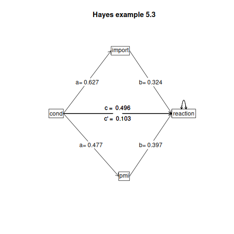
It is trivial to show the effect of multiple mediators. Do this by adding the second (or third) mediator into the equation. Use the Tal_Or data set (Tal-Or et al., 2010) again. Show the graphical representation in Figure 13.
> mod5.4 <- mediate(reaction ~ cond + (import) + (pmi), data = Tal_Or)> print(mod5.4, digits=4) #to compare with Hayes
Mediation/Moderation AnalysisCall: mediate(y = reaction ~ cond + (import) + (pmi), data = Tal_Or)The DV (Y) was reaction . The IV (X) was cond . The mediating variable(s) = import pmi .Total effect(c) of cond on reaction = 0.4957 S.E. = 0.2775 t = 1.786 df= 121 with p = 0.07661Direct effect (c') of cond on reaction removing import pmi = 0.1034 S.E. = 0.2391 t = 0.4324 df= 119 with p = 0.6662Indirect effect (ab) of cond on reaction through import pmi = 0.3923Mean bootstrapped indirect effect = 0.3926 with standard error = 0.1659 Lower CI = 0.0857 Upper CI = 0.7415R = 0.5702 R2 = 0.3251 F = 19.1118 on 3 and 119 DF p-value: 3.6636e-12 To see the longer output, specify short = FALSE in the print statement or ask for the summary
>
pdf 2
4.3 Serial mediators
The example from Hayes (2013) for two mediators, where one effects the second, is a bit more complicated and currently can be done by combining two separate analyses. The first is just model 5.4, the second is the effect of cond on pmi mediated by import.
Combining the two results leads to the output found on (Hayes, 2013, page 153).
pdf 2
> #model 5.4 + mod5.7 is the two chained mediator model> mod5.7 <- mediate(pmi ~ cond + (import) , data = Tal_Or)> summary(mod5.7, digits=4)
Call: mediate(y = pmi ~ cond + (import), data = Tal_Or)Direct effect estimates (traditional regression) (c') X + M on Y pmi se t df ProbIntercept 4.6104 0.3057 15.0836 120 1.7543e-29cond 0.3536 0.2325 1.5207 120 1.3096e-01import 0.1961 0.0671 2.9228 120 4.1467e-03R = 0.3114 R2 = 0.097 F = 6.4428 on 2 and 120 DF p-value: 0.0021989 Total effect estimates (c) (X on Y) pmi se t df ProbIntercept 5.3769 0.1618 33.2222 121 1.1593e-62cond 0.4765 0.2357 2.0218 121 4.5401e-02 'a' effect estimates (X on M) import se t df ProbIntercept 3.9077 0.2127 18.3704 121 8.3936e-37cond 0.6268 0.3098 2.0234 121 4.5235e-02 'b' effect estimates (M on Y controlling for X) pmi se t df Probimport 0.1961 0.0671 2.9228 120 0.0041467 'ab' effect estimates (through all mediators) pmi boot sd lower uppercond 0.1229 0.1271 0.084 6e-04 0.3213
4.4 Single mediators, multiple covariates
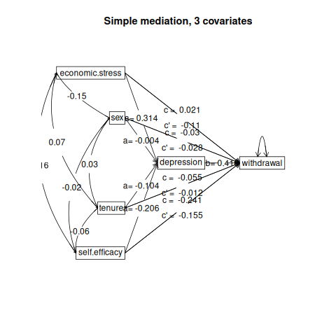
The Pollack data set (Pollack et al., 2012) is used as an example of multiple covariates (included in psychTools as a correlation matrix). The raw data are available from the processR package as estress. Confidence in executive decision making (“Entrepeneurial self-effiicacy), gender (sex), and length of time in business (tenure) are used as covariates. There are two ways of doing this: enter them as predictors of the criterion or to partial them out. The first approach estimates their effects, the second just removes them.
> lowerMat(Pollack)
sex age tenur slf.f cmptn scl.t ecnm. dprss wthdrsex 1.00age 0.07 1.00tenure 0.03 0.32 1.00self.efficacy -0.02 -0.09 -0.06 1.00competence 0.08 0.01 0.02 0.22 1.00social.ties 0.07 -0.06 0.01 0.19 0.13 1.00economic.stress -0.15 0.09 0.07 -0.16 -0.09 -0.07 1.00depression -0.05 -0.02 -0.07 -0.25 0.06 -0.05 0.34 1.00withdrawal -0.03 -0.05 -0.04 -0.24 -0.09 0.01 0.06 0.42 1.00
> mod6.2 <- mediate(withdrawal ~ economic.stress + self.efficacy + sex + tenure + (depression),+ data=Pollack, n.obs=262)> summary(mod6.2)
Call: mediate(y = withdrawal ~ economic.stress + self.efficacy + sex + tenure + (depression), data = Pollack, n.obs = 262)Direct effect estimates (traditional regression) (c') X + M on Y withdrawal se t df ProbIntercept 0.00 0.06 0.00 256 1.00e+00economic.stress -0.11 0.06 -1.82 256 6.99e-02self.efficacy -0.15 0.06 -2.67 256 8.01e-03sex -0.03 0.06 -0.50 256 6.15e-01tenure -0.01 0.06 -0.21 256 8.37e-01depression 0.42 0.06 6.83 256 6.05e-11R = 0.45 R2 = 0.21 F = 13.35 on 5 and 256 DF p-value: 1.45e-11 Total effect estimates (c) (X on Y) withdrawal se t df ProbIntercept 0.00 0.06 0.00 257 1.000000economic.stress 0.02 0.06 0.34 257 0.737000self.efficacy -0.24 0.06 -3.92 257 0.000113sex -0.03 0.06 -0.49 257 0.624000tenure -0.05 0.06 -0.91 257 0.366000 'a' effect estimates (X on M) depression se t df ProbIntercept 0.00 0.06 0.00 257 1.00e+00economic.stress 0.31 0.06 5.36 257 1.88e-07self.efficacy -0.21 0.06 -3.56 257 4.36e-04sex 0.00 0.06 -0.07 257 9.46e-01tenure -0.10 0.06 -1.82 257 6.98e-02 'b' effect estimates (M on Y controlling for X) withdrawal se t df Probdepression 0.42 0.06 6.83 256 6.05e-11 'ab' effect estimates (through all mediators) withdrawal boot sd lower uppereconomic.stress 0.13 0.09 0.03 0.04 0.14self.efficacy -0.09 -0.07 0.03 -0.12 -0.02sex 0.00 -0.01 0.02 -0.06 0.04tenure -0.04 0.00 0.02 -0.05 0.04
pdf 2
The graphical output (Figure 14) looks a bit more complicated than the figure in (Hayes, 2013, p 177) because I am showing the covariates as causal paths.
4.5 Single predictor, single criterion, multiple covariates
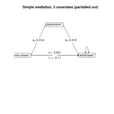
An alternative way to display the previous results is to remove the three covariates from the mediation model. Do this by partialling out the covariates. This is represented in the mediate code by a negative sign (Figure 15)
> mod6.2a <- mediate(withdrawal ~ economic.stress -self.efficacy - sex - tenure + (depression),+ data=Pollack, n.obs=262)> summary(mod6.2a)
Call: mediate(y = withdrawal ~ economic.stress - self.efficacy - sex - tenure + (depression), data = Pollack, n.obs = 262)Direct effect estimates (traditional regression) (c') X + M on Y withdrawal* se t df ProbIntercept 0.00 0.06 0.00 256 1.00e+00economic.stress -0.11 0.06 -1.80 256 7.23e-02depression 0.42 0.06 6.78 256 8.50e-11R = 0.39 R2 = 0.15 F = 23.41 on 2 and 256 DF p-value: 4.6e-10 Total effect estimates (c) (X on Y) withdrawal* se t df ProbIntercept 0.00 0.06 0.00 257 1.000economic.stress 0.02 0.06 0.34 257 0.737 'a' effect estimates (X on M) depression se t df ProbIntercept 0.00 0.06 0.00 257 1.00e+00economic.stress 0.31 0.06 5.36 257 1.88e-07 'b' effect estimates (M on Y controlling for X) withdrawal* se t df Probdepression 0.42 0.06 6.83 256 6.05e-11 'ab' effect estimates (through all mediators) withdrawal* boot sd lower uppereconomic.stress 0.13 0.12 0.03 0.06 0.18
pdf 2
4.6 Multiple predictors, single criterion
It is straightforward to use multiple predictors see (Hayes, 2013, p196) and in fact did so in the previous example where the predictors were treated as covariates. mediate also allows for multiple criteria.
5 Mediation and moderation
We already saw how to do moderation in the discussion of lmCor. Combining the concepts of mediation with moderation is done in mediate. That is, find the linear model of product terms as they are associated with dependent variables and regressed on the mediating variables.
The Garcia data set (Garcia et al., 2010) can be used for an example of moderation. (This was taken from (Hayes, 2013) but is used with kind permission of Donna M. Garcia, Michael T. Schmitt, Nyla R. Branscombe, and Naomi Ellemers.) Just as setCor and lm will find the interaction term by forming a product, so will mediate. Notice that by default, lmCor reports zero centered and standardized regressions, mediate reports zero centered but not standardized regressions, and some of the examples from Hayes (2013) do not zero center the data. Thus, I specify zero=FALSE to get the Hayes (2013) results.
It is important to note that the protest data set discussed here is from the 2013 examples and not the more recent 2018 examples available from afhayes.com. The 2013 data have a dichotomous protest variable, while the 2018 data set has three levels for the protest variable. The Garcia data set is composed of the 2018 data set with the addition of a dichotomous variable (prot2) to match the 2013 examples.
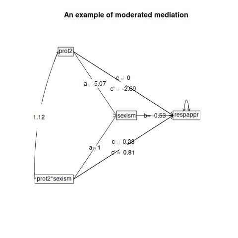
We consider how the interaction of sexism with protest affects the mediation effect of sexism (Hayes, 2013, p 362), I contrast the lm, lmCor and mediate approaches. For reasons to be discussed in the next section, I do not zero center the variables. The graphic output is in Figure 16 and the output is below. For comparison purposes, I show the results from the lm as well as lmCor and mediate.
> summary(lm(respappr ~ prot2 * sexism,data = Garcia)) #show the lm results for comparison
Call:lm(formula = respappr ~ prot2 * sexism, data = Garcia)Residuals: Min 1Q Median 3Q Max-3.4984 -0.7540 0.0801 0.8301 3.1853Coefficients: Estimate Std. Error t value Pr(>|t|)(Intercept) 6.5667 1.2095 5.429 2.83e-07 ***prot2 -2.6866 1.4515 -1.851 0.06654 .sexism -0.5290 0.2359 -2.243 0.02668 *prot2:sexism 0.8100 0.2819 2.873 0.00478 **---Signif. codes: 0 ‘***’ 0.001 ‘**’ 0.01 ‘*’ 0.05 ‘.’ 0.1 ‘ ’ 1Residual standard error: 1.144 on 125 degrees of freedomMultiple R-squared: 0.2962,Adjusted R-squared: 0.2793F-statistic: 17.53 on 3 and 125 DF, p-value: 1.456e-09
> #show the lmCor analysis> lmCor(respappr ~ prot2* sexism ,data=Garcia,zero=FALSE,main="Moderation",std=FALSE)
Call: lmCor(y = respappr ~ prot2 * sexism, data = Garcia, std = FALSE, main = "Moderation", zero = FALSE)Multiple Regression from raw data DV = respappr slope se t p lower.ci upper.ci VIF Vy.x r(Intercept) 6.57 1.21 5.43 2.8e-07 4.17 8.96 1.00 0.00 0.00prot2 -2.69 1.45 -1.85 6.7e-02 -5.56 0.19 44.99 -0.47 0.31sexism -0.53 0.24 -2.24 2.7e-02 -1.00 -0.06 3.34 -0.01 0.04prot2*sexism 0.81 0.28 2.87 4.8e-03 0.25 1.37 48.14 0.77 1.74Residual Standard Error = 1.14 with 125 degrees of freedom Multiple Regression R R2 Ruw R2uw Shrunken R2 SE of R2 overall F df1 df2 prespappr 0.54 0.3 0.45 0.2 0.28 0.06 17.53 3 125 1.46e-09
> #then show the mediate results>> modgarcia <-mediate(respappr ~ prot2 * sexism +(sexism),data=Garcia,zero=FALSE,main="Moderated mediation")> summary(modgarcia)
Call: mediate(y = respappr ~ prot2 * sexism + (sexism), data = Garcia, zero = FALSE, main = "Moderated mediation")Direct effect estimates (traditional regression) (c') X + M on Y respappr se t df ProbIntercept 6.57 1.21 5.43 125 2.83e-07prot2 -2.69 1.45 -1.85 125 6.65e-02prot2*sexism 0.81 0.28 2.87 125 4.78e-03sexism -0.53 0.24 -2.24 125 2.67e-02R = 0.54 R2 = 0.3 F = 17.53 on 3 and 125 DF p-value: 1.46e-09 Total effect estimates (c) (X on Y) respappr se t df ProbIntercept 3.88 0.18 21.39 126 9.14e-44prot2 0.00 0.84 0.00 126 9.96e-01prot2*sexism 0.28 0.16 1.79 126 7.56e-02 'a' effect estimates (X on M) sexism se t df ProbIntercept 5.07 0.07 75.12 126 1.69e-106prot2 -5.07 0.31 -16.33 126 6.81e-33prot2*sexism 1.00 0.06 17.15 126 9.41e-35 'b' effect estimates (M on Y controlling for X) respappr se t df Probsexism -0.53 0.24 -2.24 125 0.0267 'ab' effect estimates (through all mediators) respappr boot sd lower upperprot2 2.68 2.66 1.59 -0.61 5.56prot2*sexism -0.53 -0.52 0.31 -1.10 0.12
>
pdf 2
5.1 To center or not to center, that is the question
We have discussed the difference between zero centering and not zero centering. Although Hayes (2013) seems to prefer not centering, some of his examples are in fact centered. So, when we examine Table 8.2 and try to replicate the regression, we need to zero center the data.
With the global warming data from Hayes (2013), the default (uncentered) regression does not reproduce his Table, but zero centering does. To this in lm requires two steps, but we can do this in lmCor with the zero=TRUE or zero=FALSE option.
> lm(govact ~ age * negemot + posemot + ideology + sex, data=globalWarm)
Call:lm(formula = govact ~ age * negemot + posemot + ideology + sex, data = globalWarm)Coefficients:(Intercept) age negemot posemot ideology sex 5.173849 -0.023879 0.119583 -0.021419 -0.211515 -0.011191age:negemot 0.006331
> # but zero center and try again> glbwarmc <-data.frame(scale(globalWarm,scale=FALSE))> lm(govact ~ age * negemot + posemot + ideology + sex, data=globalWarm)
Call:lm(formula = govact ~ age * negemot + posemot + ideology + sex, data = globalWarm)Coefficients:(Intercept) age negemot posemot ideology sex 5.173849 -0.023879 0.119583 -0.021419 -0.211515 -0.011191age:negemot 0.006331
> mod.glb <- lmCor(govact ~ age * negemot + posemot + ideology + sex, data=globalWarm,zero=FALSE,std=FALSE)> print(mod.glb,digits=6)
Call: lmCor(y = govact ~ age * negemot + posemot + ideology + sex, data = globalWarm, std = FALSE, zero = FALSE)Multiple Regression from raw data DV = govact slope se t p lower.ci upper.ci(Intercept) 5.173849 0.338451 15.286838 1.58157e-46 4.509502 5.838197age -0.023879 0.005980 -3.992944 7.12038e-05 -0.035618 -0.012140negemot 0.119583 0.082535 1.448881 1.47759e-01 -0.042425 0.281591posemot -0.021419 0.027904 -0.767597 4.42951e-01 -0.076193 0.033354ideology -0.211515 0.026833 -7.882678 1.03603e-14 -0.264185 -0.158845sex -0.011191 0.076003 -0.147240 8.82979e-01 -0.160378 0.137997age*negemot 0.006331 0.001543 4.103542 4.48155e-05 0.003302 0.009359 VIF Vy.x r(Intercept) 1.000000 0.000000 0.000000age 6.949401 0.027844 -2.158128negemot 11.594520 0.077620 1.201328posemot 1.028663 -0.000912 0.078824ideology 1.198910 0.098323 -0.860339sex 1.052907 0.000406 -0.067105age*negemot 16.455422 0.197526 57.746593Residual Standard Error = 1.056984 with 808 degrees of freedom Multiple Regression R R2 Ruw R2uw Shrunken R2 SE of R2 overall F df1govact 0.633093 0.400806 0.14797 0.021895 0.396357 0.026299 90.07983 6 df2 pgovact 808 1.824604e-86
> mod.glb0 <- lmCor(govact ~ age * negemot + posemot + ideology + sex, data=globalWarm,std=FALSE)> print(mod.glb0,digits=6)
Call: lmCor(y = govact ~ age * negemot + posemot + ideology + sex, data = globalWarm, std = FALSE)Multiple Regression from raw data DV = govact slope se t p lower.ci upper.ci(Intercept) 4.595973 0.037089 123.916910 0.00000e+00 4.523171 4.668776age -0.001354 0.002348 -0.576864 5.64192e-01 -0.005963 0.003254negemot 0.433184 0.026243 16.506679 5.75775e-53 0.381671 0.484696posemot -0.021419 0.027904 -0.767597 4.42951e-01 -0.076193 0.033354ideology -0.211515 0.026833 -7.882678 1.03603e-14 -0.264185 -0.158845sex -0.011191 0.076003 -0.147240 8.82979e-01 -0.160378 0.137997age*negemot 0.006331 0.001543 4.103542 4.48155e-05 0.003302 0.009359 VIF Vy.x r(Intercept) 1.000000 0.000000 0.000000age 1.071058 0.001579 -2.158128negemot 1.172207 0.281175 1.201328posemot 1.028663 -0.000912 0.078824ideology 1.198910 0.098323 -0.860339sex 1.052907 0.000406 -0.067105age*negemot 1.014744 0.020236 5.915986Residual Standard Error = 1.056984 with 808 degrees of freedom Multiple Regression R R2 Ruw R2uw Shrunken R2 SE of R2 overall F df1govact 0.633093 0.400806 0.074427 0.005539 0.396357 0.026299 90.07983 6 df2 pgovact 808 1.824604e-86
So, when we do the mediated moderation model, we need to use the zero centered option to match the Hayes (2013) results from Figure 8.5.
> #by default, mediate zero centers before finding the products> mod.glb <- mediate(govact ~ age * negemot + posemot + ideology + sex + (age), data=globalWarm,zero=TRUE)> summary(mod.glb,digits=4)
Call: mediate(y = govact ~ age * negemot + posemot + ideology + sex + (age), data = globalWarm, zero = TRUE)Direct effect estimates (traditional regression) (c') X + M on Y govact se t df ProbIntercept 0.0090 0.0371 0.2421 808 8.0876e-01negemot 0.4332 0.0262 16.5067 808 5.7578e-53posemot -0.0214 0.0279 -0.7676 808 4.4295e-01ideology -0.2115 0.0268 -7.8827 808 1.0360e-14sex -0.0112 0.0760 -0.1472 808 8.8298e-01age*negemot 0.0063 0.0015 4.1035 808 4.4816e-05age -0.0014 0.0023 -0.5769 808 5.6419e-01R = 0.6331 R2 = 0.4008 F = 90.0798 on 6 and 808 DF p-value: 1.8246e-86 Total effect estimates (c) (X on Y) govact se t df ProbIntercept 0.0090 0.0371 0.2420 809 8.0881e-01negemot 0.4328 0.0262 16.5043 809 5.8181e-53posemot -0.0220 0.0279 -0.7890 809 4.3036e-01ideology -0.2145 0.0263 -8.1510 809 1.3690e-15sex -0.0173 0.0752 -0.2304 809 8.1783e-01age*negemot 0.0063 0.0015 4.1025 809 4.4999e-05 'a' effect estimates (X on M) age se t df ProbIntercept 0.0044 0.5554 0.0079 809 9.9366e-01negemot 0.2757 0.3929 0.7017 809 4.8305e-01posemot 0.4232 0.4176 1.0135 809 3.1112e-01ideology 2.2079 0.3943 5.6002 809 2.9334e-08sex 4.5345 1.1269 4.0238 809 6.2643e-05age*negemot 0.0031 0.0231 0.1346 809 8.9294e-01 'b' effect estimates (M on Y controlling for X) govact se t df Probage -0.0014 0.0023 -0.5769 808 0.56419 'ab' effect estimates (through all mediators) govact boot sd lower uppernegemot -0.0004 -0.0004 0.0012 -0.0033 0.0016posemot -0.0006 -0.0006 0.0015 -0.0040 0.0020ideology -0.0030 -0.0030 0.0051 -0.0134 0.0066sex -0.0061 -0.0059 0.0106 -0.0285 0.0137age*negemot 0.0000 0.0000 0.0001 -0.0002 0.0002
Compare this output to that of Table 8.2 and Figure 8.5 (p 258 - 259).
5.2 Another example of moderated mediation
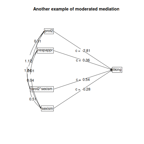
The Garcia data set (protest in Hayes (2013)) is another example of a moderated analysis. Use either lmCor or mediate to examine this data set. The defaults for these two differ, in that lmCor assumes we want to zero center and standardize, while mediate defaults to not standardizing but also defaults to zero (mean) centering. Note that in the next examples we specify we do not want to standardize nor to mean center.
> psych::describe(Garcia)
vars n mean sd median trimmed mad min max range skew kurtosisprotest 1 129 1.03 0.82 1.00 1.04 1.48 0.00 2 2.00 -0.06 -1.52sexism 2 129 5.12 0.78 5.12 5.10 0.74 2.87 7 4.13 0.12 -0.32anger 3 129 2.12 1.66 1.00 1.84 0.00 1.00 7 6.00 1.29 0.26liking 4 129 5.64 1.05 5.83 5.73 0.99 1.00 7 6.00 -1.15 2.48respappr 5 129 4.87 1.35 5.25 4.98 1.11 1.50 7 5.50 -0.75 -0.18prot2 6 129 0.68 0.47 1.00 0.72 0.00 0.00 1 1.00 -0.77 -1.41 seprotest 0.07sexism 0.07anger 0.15liking 0.09respappr 0.12prot2 0.04
> lm(liking ~ prot2* sexism + respappr, data=Garcia)
Call:lm(formula = liking ~ prot2 * sexism + respappr, data = Garcia)Coefficients: (Intercept) prot2 sexism respappr prot2:sexism 5.3471 -2.8075 -0.2824 0.3593 0.5426
> lmCor(liking ~ prot2* sexism + respappr, data = Garcia, zero=FALSE,std=FALSE)
Call: lmCor(y = liking ~ prot2 * sexism + respappr, data = Garcia, std = FALSE, zero = FALSE)Multiple Regression from raw data DV = liking slope se t p lower.ci upper.ci VIF Vy.x r(Intercept) 5.35 1.06 5.04 1.6e-06 3.25 7.45 1.00 0.00 0.00prot2 -2.81 1.16 -2.42 1.7e-02 -5.10 -0.51 46.22 -0.27 0.10sexism -0.28 0.19 -1.49 1.4e-01 -0.66 0.09 3.47 -0.02 0.08respappr 0.36 0.07 5.09 1.3e-06 0.22 0.50 1.42 0.23 0.70prot2*sexism 0.54 0.23 2.36 2.0e-02 0.09 1.00 51.32 0.34 0.69Residual Standard Error = 0.9 with 124 degrees of freedom Multiple Regression R R2 Ruw R2uw Shrunken R2 SE of R2 overall F df1 df2 pliking 0.53 0.28 0.36 0.13 0.26 0.06 12.26 4 124 1.99e-08
> mod7.4 <- mediate(liking ~ prot2 * sexism +respappr, data = Garcia, zero=FALSE)> summary(mod7.4)
Call: mediate(y = liking ~ prot2 * sexism + respappr, data = Garcia, zero = FALSE)No mediator specified leads to traditional regression liking se t df ProbIntercept 5.35 1.06 5.04 124 1.60e-06prot2 -2.81 1.16 -2.42 124 1.70e-02sexism -0.28 0.19 -1.49 124 1.39e-01respappr 0.36 0.07 5.09 124 1.28e-06prot2*sexism 0.54 0.23 2.36 124 1.97e-02R = 0.53 R2 = 0.28 F = 12.26 on 4 and 124 DF p-value: 1.99e-08
pdf 2
5.3 Graphic Displays of Interactions
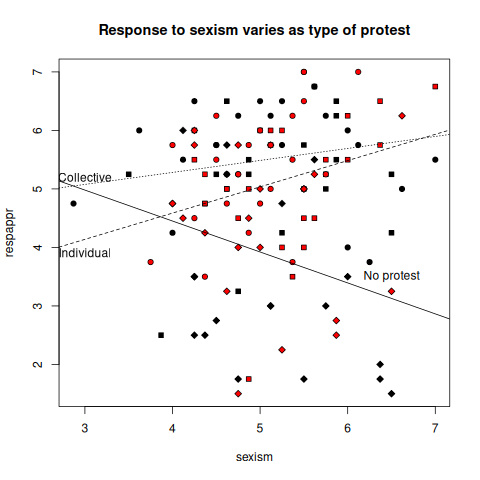
In order to graphically display interactions, particularly if one of the variable is categorical, pllot separate regression lines for each value of the categorical variable. Do this for the Garcia data set to show the interaction of protest with sexism. (see Figure 18). This is just an example of how to use Core-R to do graphics and is not a feature of psych.
> png('garciainteraction.png')> plot(respappr ~ sexism, pch = 23- protest, bg = c("black","red", "blue")[protest],+ data=Garcia, main = "Response to sexism varies as type of protest")> by(Garcia,Garcia$protest, function(x) abline(lm(respappr ~ sexism,+ data =x),lty=c("solid","dashed","dotted")[x$protest+1]))
Garcia$protest: 0NULL------------------------------------------------------------Garcia$protest: 1NULL------------------------------------------------------------Garcia$protest: 2NULL
> text(6.5,3.5,"No protest")> text(3,3.9,"Individual")> text(3,5.2,"Collective")> dev.off()
pdf 2
>
6 Partial Correlations
Although not strickly speaking part of mediation or moderation, the use of partial correlations can be addressed here. s
6.1 Partial some variables from the rest of the variables
Given a set of X variables and a set of Y variables, we can control for an additional set of Z variables when we find the correlations between X and Y. This is effectively what happens when we want to add covariates into a model. We see this when we compare the regression model for government action as a function of the iteraction of ideology and age with some covariates, or when we partial them out first.
> #first, the more complicated model> mod.glb <- lmCor(govact ~ age * negemot + posemot + ideology + sex,+ data=globalWarm,std=FALSE)> print(mod.glb,digits=3)
Call: lmCor(y = govact ~ age * negemot + posemot + ideology + sex, data = globalWarm, std = FALSE)Multiple Regression from raw data DV = govact slope se t p lower.ci upper.ci VIF Vy.x r(Intercept) 4.596 0.037 123.917 0.00e+00 4.523 4.669 1.000 0.000 0.000age -0.001 0.002 -0.577 5.64e-01 -0.006 0.003 1.071 0.002 -2.158negemot 0.433 0.026 16.507 5.76e-53 0.382 0.485 1.172 0.281 1.201posemot -0.021 0.028 -0.768 4.43e-01 -0.076 0.033 1.029 -0.001 0.079ideology -0.212 0.027 -7.883 1.04e-14 -0.264 -0.159 1.199 0.098 -0.860sex -0.011 0.076 -0.147 8.83e-01 -0.160 0.138 1.053 0.000 -0.067age*negemot 0.006 0.002 4.104 4.48e-05 0.003 0.009 1.015 0.020 5.916Residual Standard Error = 1.057 with 808 degrees of freedom Multiple Regression R R2 Ruw R2uw Shrunken R2 SE of R2 overall F df1 df2 pgovact 0.633 0.401 0.074 0.006 0.396 0.026 90.08 6 808 1.825e-86
> # compare this to the partialled model>> mod.glb.partialled <- lmCor(govact ~ age * negemot - posemot - ideology - sex,data = globalWarm)>
Note how the beta weights for the age, negemot and interaction terms are identical.
6.2 Partial everything from everything
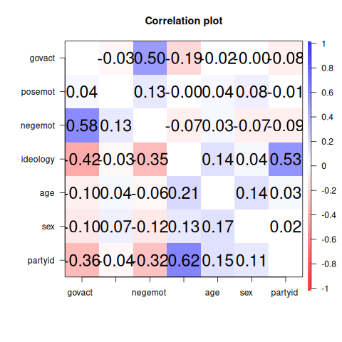
Sometimes we want to examine just the independent effects of all our variables. That is to say, we want to partial all the variables from all the other variables. I do this with the partial.r function. To show the results, I compare the partialed rs to the original rs. I show the lower off diagonal matrix using lowerMat. Then to compare the partial matrix to the original matrix, I form the square matrix where the lower off diagonal is the original matrix and the upper off diagonal is the partial matrix.
> upper <-partial.r(globalWarm)> lowerMat(upper) #show it
govct posmt negmt idlgy age sex prtydgovact 1.00posemot -0.03 1.00negemot 0.50 0.13 1.00ideology -0.19 0.00 -0.07 1.00age -0.02 0.04 0.03 0.14 1.00sex 0.00 0.08 -0.07 0.04 0.14 1.00partyid -0.08 -0.01 -0.09 0.53 0.03 0.02 1.00
> lower <- lowerCor(globalWarm)
govct posmt negmt idlgy age sex prtydgovact 1.00posemot 0.04 1.00negemot 0.58 0.13 1.00ideology -0.42 -0.03 -0.35 1.00age -0.10 0.04 -0.06 0.21 1.00sex -0.10 0.07 -0.12 0.13 0.17 1.00partyid -0.36 -0.04 -0.32 0.62 0.15 0.11 1.00
> lowup <- lowerUpper(lower,upper)>
pdf 2
7 Related packages
mediate and lmCor are just two functions in the psych package. There are several additional packages available in R to do mediation. The mediation package (Tingley et al., 2014) seems the most powerful, in that is tailor made for mediation. MBESS (Kelley, 2017) has a mediation function. Steven Short has a nice tutorial on mediation analysis available for download that discusses how to use R for mediation. And, of course, the lavaan package (Rosseel, 2012) is the recommended package to do SEM and path models.
8 Development version and a users guide
The psych package is available from the CRAN repository. However, the most recent development version of the psych package is available as a source file at the repository maintained at https://personality-project.org/r/. That version will have removed the most recently discovered bugs (but perhaps introduced other, yet to be discovered ones). To install this development version, either for PCs or Macs,
install.packages("psych", repos = "https://personality-project.org/r", type = "source")
After doing this, it is important to restart R to get the new package.
Although the individual help pages for the psych package are available as part of R and may be accessed directly (e.g. ?psych) , the full manual for the psych package is also available as a pdf at https://personality-project.org/r/psych-manual.pdf
News and a history of changes are available in the NEWS and CHANGES files in the source files. To view the most recent news,
> news(Version >= "2.6.1",package="psych")
9 Psychometric Theory
The psych package has been developed to help psychologists (and other quantitative scientists) do basic research. Many of the functions were developed to supplement a book (http://personality-project.org/r/book/ An introduction to Psychometric Theory with Applications in R (Revelle, prep) More information about the use of some of the functions may be found in the book .
For more extensive discussion of the use of psych in particular and R in general, consult http://personality-project.org/r/r.guide.html A short guide to R.
10 SessionInfo
This document was prepared using the following settings.
> sessionInfo()
R version 4.6.2 (2026-10-29)Platform: x86_64-pc-linux-gnuRunning under: Ubuntu 26.04.1 LTSMatrix products: defaultBLAS: /usr/lib/x86_64-linux-gnu/blas/libblas.so.3.12.1LAPACK: /usr/lib/x86_64-linux-gnu/lapack/liblapack.so.3.12.1; LAPACK version 3.12.0locale: [1] LC_CTYPE=C.UTF-8 LC_NUMERIC=C LC_TIME=C.UTF-8 [4] LC_COLLATE=C.UTF-8 LC_MONETARY=C.UTF-8 LC_MESSAGES=C.UTF-8 [7] LC_PAPER=C.UTF-8 LC_NAME=C LC_ADDRESS=C[10] LC_TELEPHONE=C LC_MEASUREMENT=C.UTF-8 LC_IDENTIFICATION=Ctime zone: Etc/UTCtzcode source: system (glibc)attached base packages:[1] stats graphics grDevices utils datasets methods baseother attached packages:[1] psychTools_2.6.4 psych_2.6.9loaded via a namespace (and not attached):[1] compiler_4.6.2 parallel_4.6.2 tools_4.6.2 foreign_0.8-92 nlme_3.1-172[6] mnormt_2.1.2 grid_4.6.2 lattice_0.23-1
References
- Cohen (1982) Cohen, J. (1982). Set correlation as a general mulitivariate data-analytic method. Multivariate Behavioral Research, 17(3):301–341.
- Cohen et al. (2003) Cohen, J., Cohen, P., West, S. G., and Aiken, L. S. (2003). Applied multiple regression/correlation analysis for the behavioral sciences. L. Erlbaum Associates, Mahwah, N.J., 3rd ed edition.
- Dawes (1979) Dawes, R. M. (1979). The robust beauty of improper linear models in decision making. American Psychologist, 34(7):571–582.
- Garcia et al. (2010) Garcia, D. M., Schmitt, M. T., Branscombe, N. R., and Ellemers, N. (2010). Women’s reactions to ingroup members who protest discriminatory treatment: The importance of beliefs about inequality and response appropriateness. European Journal of Social Psychology, 40(5):733–745.
- Hayes (2013) Hayes, A. F. (2013). Introduction to mediation, moderation, and conditional process analysis: A regression-based approach. Guilford Press, New York.
- Hotelling (1936) Hotelling, H. (1936). Relations between two sets of variates. Biometrika, 28(3/4):321–377.
- Kelley (2017) Kelley, K. (2017). MBESS: The MBESS R Package. R package version 4.4.1.
- Pollack et al. (2012) Pollack, J. M., Vanepps, E. M., and Hayes, A. F. (2012). The moderating role of social ties on entrepreneurs’ depressed affect and withdrawal intentions in response to economic stress. Journal of Organizational Behavior, 33(6):789–810.
- Preacher (2015) Preacher, K. J. (2015). Advances in mediation analysis: A survey and synthesis of new developments. Annual Review of Psychology, 66:825–852.
- Preacher and Hayes (2004) Preacher, K. J. and Hayes, A. F. (2004). SPSS and SAS procedures for estimating indirect effects in simple mediation models. Behavior Research Methods, Instruments, & Computers, 36(4):717–731.
- Preacher et al. (2007) Preacher, K. J., Rucker, D. D., and Hayes, A. F. (2007). Addressing moderated mediation hypotheses: Theory, methods, and prescriptions. Multivariate behavioral research, 42(1):185–227.
- R Core Team (2025) R Core Team (2025). R: A Language and Environment for Statistical Computing. R Foundation for Statistical Computing, Vienna, Austria.
- Revelle (2026) Revelle, W. (2023). psych: Procedures for Personality and Psychological Research. Northwestern University, Evanston, https://CRAN.r-project.org/package=psych. R package version 2.6.4
- Revelle (prep) Revelle, W. (in prep). An introduction to psychometric theory with applications in R. Springer.
- Rosseel (2012) Rosseel, Y. (2012). lavaan: An R package for structural equation modeling. Journal of Statistical Software, 48(2):1–36.
- Tal-Or et al. (2010) Tal-Or, N., Cohen, J., Tsfati, Y., and Gunther, A. C. (2010). Testing causal direction in the influence of presumed media influence. Communication Research, 37(6):801–824.
- Tingley et al. (2014) Tingley, D., Yamamoto, T., Hirose, K., Keele, L., and Imai, K. (2014). mediation: R package for causal mediation analysis. Journal of Statistical Software, 59(5):1–38.
References
- Cohen (1982) Cohen, J. (1982). Set correlation as a general mulitivariate data-analytic method. Multivariate Behavioral Research, 17(3):301–341.
- Cohen et al. (2003) Cohen, J., Cohen, P., West, S. G., and Aiken, L. S. (2003). Applied multiple regression/correlation analysis for the behavioral sciences. L. Erlbaum Associates, Mahwah, N.J., 3rd ed edition.
- Dawes (1979) Dawes, R. M. (1979). The robust beauty of improper linear models in decision making. American Psychologist, 34(7):571–582.
- Garcia et al. (2010) Garcia, D. M., Schmitt, M. T., Branscombe, N. R., and Ellemers, N. (2010). Women’s reactions to ingroup members who protest discriminatory treatment: The importance of beliefs about inequality and response appropriateness. European Journal of Social Psychology, 40(5):733–745.
- Hayes (2013) Hayes, A. F. (2013). Introduction to mediation, moderation, and conditional process analysis: A regression-based approach. Guilford Press, New York.
- Hotelling (1936) Hotelling, H. (1936). Relations between two sets of variates. Biometrika, 28(3/4):321–377.
- Kelley (2017) Kelley, K. (2017). MBESS: The MBESS R Package. R package version 4.4.1.
- Pollack et al. (2012) Pollack, J. M., Vanepps, E. M., and Hayes, A. F. (2012). The moderating role of social ties on entrepreneurs’ depressed affect and withdrawal intentions in response to economic stress. Journal of Organizational Behavior, 33(6):789–810.
- Preacher (2015) Preacher, K. J. (2015). Advances in mediation analysis: A survey and synthesis of new developments. Annual Review of Psychology, 66:825–852.
- Preacher and Hayes (2004) Preacher, K. J. and Hayes, A. F. (2004). SPSS and SAS procedures for estimating indirect effects in simple mediation models. Behavior Research Methods, Instruments, & Computers, 36(4):717–731.
- Preacher et al. (2007) Preacher, K. J., Rucker, D. D., and Hayes, A. F. (2007). Addressing moderated mediation hypotheses: Theory, methods, and prescriptions. Multivariate behavioral research, 42(1):185–227.
- R Core Team (2023) R Core Team (2023). R: A Language and Environment for Statistical Computing. R Foundation for Statistical Computing, Vienna, Austria.
- Moon (2020) Keon-Woong Moon (2020). processR: Implementation of the ’PROCESS’ Macro. https://CRAN.R-project.org/package=processR
- Revelle (2025) Revelle, W. (2025). psych: Procedures for Personality and Psychological Research. Northwestern University, Evanston, https://CRAN.r-project.org/package=psych. R package version 2.4.3
- Revelle (prep) Revelle, W. (in prep). An introduction to psychometric theory with applications in R. Springer.
- Rosseel (2012) Rosseel, Y. (2012). lavaan: An R package for structural equation modeling. Journal of Statistical Software, 48(2):1–36.
- Tabachnick and Fidell (2001) Tabacnik, B.G and Fidell, L.S. (2001) Using multivariate statistics. Allyn and Bacon.
- Tal-Or et al. (2010) Tal-Or, N., Cohen, J., Tsfati, Y., and Gunther, A. C. (2010). Testing causal direction in the influence of presumed media influence. Communication Research, 37(6):801–824.
- Tingley et al. (2014) Tingley, D., Yamamoto, T., Hirose, K., Keele, L., and Imai, K. (2014). mediation: R package for causal mediation analysis. Journal of Statistical Software, 59(5):1–38.